[Update 2017.06.11] Add chainer v2 code
Writing your CNN model
This is example of small Convolutional Neural Network definition, CNNSmall
import chainer
import chainer.functions as F
import chainer.links as L


class CNNSmall(chainer.Chain):
    def __init__(self, n_out):
        super(CNNSmall, self).__init__()
        with self.init_scope():
            self.conv1 = L.Convolution2D(None, 16, 3, 2)
            self.conv2 = L.Convolution2D(16, 32, 3, 2)
            self.conv3 = L.Convolution2D(32, 32, 3, 2)
            self.fc4 = L.Linear(None, 100)
            self.fc5 = L.Linear(100, n_out)

    def __call__(self, x):
        h = F.relu(self.conv1(x))
        h = F.relu(self.conv2(h))
        h = F.relu(self.conv3(h))
        h = F.relu(self.fc4(h))
        h = self.fc5(h)
        return h
I also made a slightly bigger CNN, called CNNMedium,
import chainer
import chainer.functions as F
import chainer.links as L


class CNNMedium(chainer.Chain):
    def __init__(self, n_out):
        super(CNNMedium, self).__init__()
        with self.init_scope():
            self.conv1 = L.Convolution2D(None, 16, 3, 1)
            self.conv2 = L.Convolution2D(16, 32, 3, 2)
            self.conv3 = L.Convolution2D(32, 32, 3, 1)
            self.conv4 = L.Convolution2D(32, 64, 3, 2)
            self.conv5 = L.Convolution2D(64, 64, 3, 1)
            self.conv6 = L.Convolution2D(64, 128, 3, 2)
            self.fc7 = L.Linear(None, 100)
            self.fc8 = L.Linear(100, n_out)

    def __call__(self, x):
        h = F.relu(self.conv1(x))
        h = F.relu(self.conv2(h))
        h = F.relu(self.conv3(h))
        h = F.relu(self.conv4(h))
        h = F.relu(self.conv5(h))
        h = F.relu(self.conv6(h))
        h = F.relu(self.fc7(h))
        h = self.fc8(h)
        return h
It is nice to know the computational cost for Convolution layer, which is approximated as,
- \( CH_I \) : Input image channel
- \( CH_O \) : Output image channel
- \( H_I \) : Input image height
- \( W_I \) : Input image width
- \( k \) : kernal size (assuming same for width & height)
In above CNN definitions, the size of the channel is bigger for deeper layer. This can be understood by calculating the computational cost for each layer.
When L.Convolution2D with stride=2 is used, the size of image become almost half. This means \( H_I\) and \( W_I \) becomes small value, so \(CH_I \) and \( CH_O \) can take larger value.
[TODO: add computational cost table for CNN Medium example]
Training CIFAR-10
Once you have written CNN, it is easy to train this model. The code, train_cifar10.py, is quite similar to MNIST training code.
Only small difference is the dataset preparation for CIFAR-10,
    # 3. Load the CIFAR-10 dataset
    train, test = chainer.datasets.get_cifar10()
and model setup
from CNNSmall import CNNSmall
from CNNMedium import CNNMedium

    archs = {
        'cnnsmall': CNNSmall,
        'cnnmedium': CNNMedium,
    }

    ...

    class_num = 10
    model = archs[args.arch](n_out=class_num)
The whole source code is the following,
from __future__ import print_function
import argparse

import chainer
import chainer.functions as F
import chainer.links as L
from chainer import training, iterators, serializers, optimizers
from chainer.training import extensions

from CNNSmall import CNNSmall
from CNNMedium import CNNMedium


def main():
    archs = {
        'cnnsmall': CNNSmall,
        'cnnmedium': CNNMedium,
    }

    parser = argparse.ArgumentParser(description='Cifar-10 CNN example')
    parser.add_argument('--arch', '-a', choices=archs.keys(),
                        default='cnnsmall', help='Convnet architecture')
    parser.add_argument('--batchsize', '-b', type=int, default=64,
                        help='Number of images in each mini-batch')
    parser.add_argument('--epoch', '-e', type=int, default=20,
                        help='Number of sweeps over the dataset to train')
    parser.add_argument('--gpu', '-g', type=int, default=-1,
                        help='GPU ID (negative value indicates CPU)')
    parser.add_argument('--out', '-o', default='result-cifar10',
                        help='Directory to output the result')
    parser.add_argument('--resume', '-r', default='',
                        help='Resume the training from snapshot')
    args = parser.parse_args()

    print('GPU: {}'.format(args.gpu))
    print('# Minibatch-size: {}'.format(args.batchsize))
    print('# epoch: {}'.format(args.epoch))
    print('')

    # 1. Setup model
    class_num = 10
    model = archs[args.arch](n_out=class_num)
    classifier_model = L.Classifier(model)
    if args.gpu >= 0:
        chainer.cuda.get_device(args.gpu).use()  # Make a specified GPU current
        classifier_model.to_gpu()  # Copy the model to the GPU

    # 2. Setup an optimizer
    optimizer = optimizers.Adam()
    optimizer.setup(classifier_model)

    # 3. Load the CIFAR-10 dataset
    train, test = chainer.datasets.get_cifar10()

    # 4. Setup an Iterator
    train_iter = iterators.SerialIterator(train, args.batchsize)
    test_iter = iterators.SerialIterator(test, args.batchsize,
                                         repeat=False, shuffle=False)

    # 5. Setup an Updater
    updater = training.StandardUpdater(train_iter, optimizer, device=args.gpu)
    # 6. Setup a trainer (and extensions)
    trainer = training.Trainer(updater, (args.epoch, 'epoch'), out=args.out)

    # Evaluate the model with the test dataset for each epoch
    trainer.extend(extensions.Evaluator(test_iter, classifier_model, device=args.gpu))

    trainer.extend(extensions.dump_graph('main/loss'))
    trainer.extend(extensions.snapshot(), trigger=(1, 'epoch'))
    trainer.extend(extensions.LogReport())
    trainer.extend(extensions.PrintReport(
        ['epoch', 'main/loss', 'validation/main/loss',
         'main/accuracy', 'validation/main/accuracy', 'elapsed_time']))
    trainer.extend(extensions.PlotReport(
        ['main/loss', 'validation/main/loss'],
        x_key='epoch', file_name='loss.png'))
    trainer.extend(extensions.PlotReport(
        ['main/accuracy', 'validation/main/accuracy'],
        x_key='epoch',
        file_name='accuracy.png'))

    trainer.extend(extensions.ProgressBar())

    # Resume from a snapshot
    if args.resume:
        serializers.load_npz(args.resume, trainer)

    # Run the training
    trainer.run()
    serializers.save_npz('{}/{}-cifar10.model'
                         .format(args.out, args.arch), model)

if __name__ == '__main__':
    main()
See how clean the code is! Chainer abstracts the training process and thus the code can be reusable with other deep learning training.
[hands on] Try running train code.
Below is example in my environment
- CNNSmall model
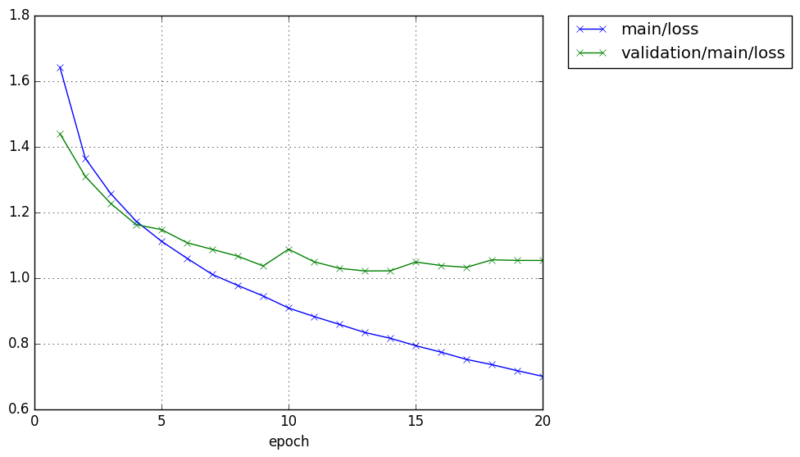
$ python train_cifar10.py -g 0 -o result-cifar10-cnnsmall -a cnnsmall
GPU: 0
# Minibatch-size: 64
# epoch: 20

epoch       main/loss   validation/main/loss  main/accuracy  validation/main/accuracy  elapsed_time
1           1.66603     1.44016               0.397638       0.477807                  6.22123
2           1.36101     1.31731               0.511324       0.527568                  12.0878
3           1.23553     1.20439               0.559119       0.568073                  17.9239
4           1.14553     1.13121               0.589609       0.595541                  23.7497
5           1.08058     1.09946               0.617747       0.606588                  29.5948
6           1.02242     1.1259                0.638784       0.605295                  35.4604
7           0.97847     1.0797                0.65533        0.615048                  41.3058
8           0.938967    1.0584                0.669494       0.621815                  47.184
9           0.902363    1.00883               0.681985       0.646099                  53.0965
10          0.872796    1.00743               0.692782       0.644904                  58.982
11          0.838787    0.993791              0.705226       0.651971                  64.9511
12          0.813549    0.987916              0.714609       0.655454                  70.3869
13          0.785552    0.987968              0.723825       0.659236                  75.8247
14          0.766127    1.0092                0.730074       0.656748                  81.4311
15          0.743967    1.04623               0.738496       0.650876                  86.9175
16          0.723779    0.991238              0.744518       0.665008                  92.6226
17          0.704939    1.02468               0.752058       0.655354                  98.1399
18          0.68687     0.999966              0.756962       0.660629                  103.657
19          0.668204    1.00803               0.763564       0.660928                  109.226
20          0.650081    1.01554               0.769906       0.667197                  114.705
Chainer extension, PlotReport will automatically create the graph of loss and accuracy for each epoch.
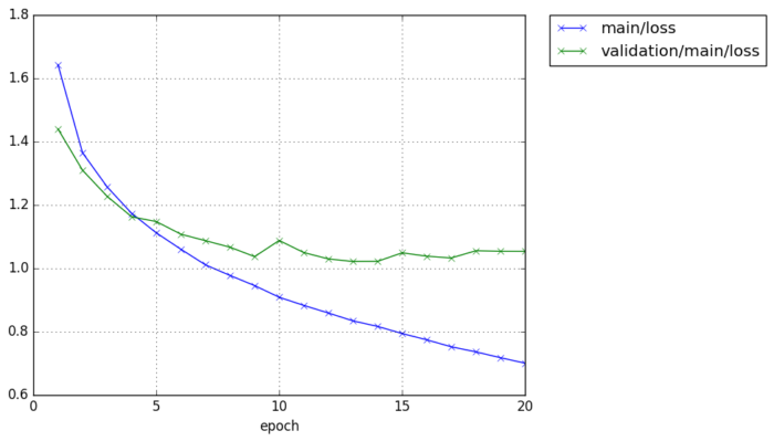
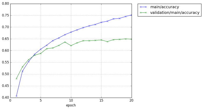
We can achieve around 65% validation accuracy with such a easy CNN construction.
- CNNMedium
$ python train_cifar10.py -g 0 -o result-cifar10-cnnmedium -a cnnmedium
GPU: 0
# Minibatch-size: 64
# epoch: 20

epoch       main/loss   validation/main/loss  main/accuracy  validation/main/accuracy  elapsed_time
1           1.62656     1.3921                0.402494       0.493133                  7.61706
2           1.31508     1.2771                0.526448       0.54588                   15.209
3           1.14961     1.12021               0.589749       0.603603                  22.7185
4           1.04442     1.05119               0.631182       0.629877                  30.1564
5           0.947944    1.00655               0.66624        0.648288                  37.8547
6           0.876341    1.0247                0.690021       0.644705                  46.9253
7           0.819997    0.983303              0.711968       0.662719                  54.9994
8           0.757557    0.933339              0.733795       0.677846                  62.4761
9           0.699673    0.948701              0.751539       0.682126                  69.8784
10          0.652811    0.965453              0.769006       0.680533                  77.2829
11          0.606698    0.990516              0.785551       0.671278                  84.6915
12          0.559568    0.999138              0.799996       0.682822                  92.068
13          0.521884    1.07451               0.814158       0.678742                  99.4703
14          0.477247    1.08184               0.829445       0.673865                  107.249
15          0.443625    1.08582               0.840109       0.680832                  114.609
16          0.406318    1.26192               0.853573       0.660529                  122.218
17          0.378328    1.2075                0.86507        0.670183                  129.655
18          0.349719    1.27795               0.87548        0.673467                  137.098
19          0.329299    1.32094               0.881702       0.664709                  144.553
20          0.297305    1.39914               0.894426       0.666202                  151.959
As expected, CNNMedium takes little bit longer time for computation but it achieves higher accuracy for training data.
※ It is also important to notice that validation accuracy is almost same between CNNSmall and CNNMedium, which means CNNMedium may be overfitting to the training data. To avoid overfitting, data augmentation (flip, rotate, clip, resize, add gaussian noise etc the input image to increase the effective data size) technique is often used in practice.
Training CIFAR-100
Again, training CIFAR-100 is quite similar to the training of CIFAR-10.
See train_cifar100.py. Only the difference is model definition to set the output class number (model definition itself is not changed and can be reused!!).
    # 1. Setup model
    class_num = 100
    model = archs[args.arch](n_out=class_num)
and dataset preparation
    # 3. Load the CIFAR-10 dataset
    train, test = chainer.datasets.get_cifar100()
[hands on] Try running train code.
Summary
We have learned how to train CNN with Chainer. CNN is widely used many image processing tasks, not only image classification. For example,
- Bounding Box detection
- SSD, YoLo V2
- Semantic segmentation
- FCN
- Colorization
- PaintsChainer
- Image generation
- GAN
- Style transfer
- chainer goph
- Super resolution
- SeRanet
etc. Now you are ready to enter these advanced image processing with deep learning!
[hands on]
Try modifying the CNN model or create your own CNN model and train it to see the computational speed and its performance (accuracy). You may try changing following
- model depth
- channel size of each layer
- Layer (Ex. use
F.max_pooling_2dinstead ofL.Convolution2Dwith stride 2) - activation function (
F.relutoF.leaky_relu,F.sigmoid,F.tanhetc…) - Try inserting another layer, Ex.
L.BatchNormalizationorF.dropout.
etc.
You can refer Chainer example codes to see the network definition examples.
Also, try configuring hyper parameter to see the performance
- Change optimizer
- Change learning rate of optimizer
etc.