Japanese is available at Qiita.

From left: 1. Classification saliency map visualization of VGG16, CNN model. 2. iris dataset feature importance calculation of MLP model. 3. Water solubility contribution visualization of Graph convolutional network model.
Abstract
Have you ever thought “Deep neural network is highly complicated black box, no one ever able to see what happens inside to result this output.”?
Even though NN consists of many layers and its mathematical analysis is difficult, there are some researches to show some saliency map like above images to understand model’s behavior or to get new knowledge for the dataset.
These saliency map calculation methods are implemented in Chainer Chemistry (even though the name contains “chemistry”, saliency module is available in many domains, as explained below). I will briefly explain how these work, and how to use it. You can also show these visualization figures after read this (a little bit long) article, enjoy!
It starts from theoretical explanation, followed by the code to use the module. Please jump to the “Examples” section if you just want to use it.
The code in this article is uploaded on github
– https://github.com/corochann/chainer-saliency
What is reasoning of NN?
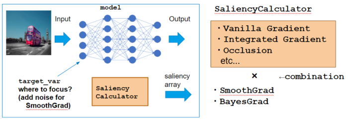
3 saliency calculation methods are implemented so far in chainer chemistry.
– VanillaGrad
– IntegratedGradient
– Occlusion
These methods calculate the contribution to the model’s prediction for each data.
※ Note that feature importance used in Random forest or XGBoost are calculated for the model. There is a difference that it is not calculated for “each data”.
Brief introduction – VanillaGrad
This method calculates derivative of output y with respect to input x, as a input contribution to the output prediction.
$$ s_i = \frac{dy}{dx_i} $$
Here, \(s_i\) is the saliency score, which is calculated for each input data’s \(i\)-th element \(x_i\). When the value of gradient is large for some element, the value change of this element results in big change of output prediction. So this element should have larger saliency (importance).
In terms of implementation, it is simply written as follows with chainer.
y = model(x)
y.backward()
s = x.grad
Saliency module usage
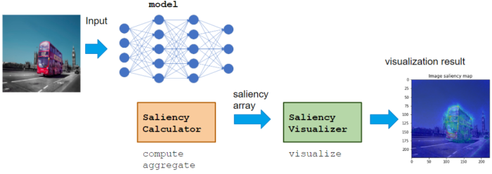
Calculator class calculates saliency score, like VaillaGrad, IntegratedGradient, or Occlusion.
Visualizer class visualizes calculated saliency score.
Calculator can be used with various NN model, which does not restrict the domain or application. Visualizer can be implemented to adopt Application for the proper visualization for the domain.
Basic usage flow is to call Calculator compute, aggregate -> Visualizer visualize
# model is chainer.Chain, x is dataset
calculator = GradientCalculator(model)
saliency_samples = calculator.compute(x)
saliency = calculator.aggregate(saliency_samples)

visualizer = ImageVisualizer()
visualizer.visualize(saliency)
Calculator class
Here I use GradientCalculator as an example which calcultes VanillaGrad explained above. Let’s see how to call each method.
Instantiation
Instance with passing model, which is the target neural network to calculate saliency.
calculator = GradientCalculator(model)
compute method
compute method calculates “saliency samples” for each data x.
# x (bs, num_feature) -> saliency_samples (M, bs, num_feature)
saliency_samples = calculator.compute(x, M=1)
Here, M samples of saliency is calculated.
When calculating VanillaGrad, it suffices with M=1 since the calculation result of grad is always same. However, sampling is necessary when we consider SmoothGrad or BayesGrad.
I will explain SmoothGrad & BayesGrad to understand the notion of sampling.
– SmoothGrad –
Practically, VanillaGrad tends to show Noisy saliency map, so SmoothGrad suggests to change
input x to shift a small ϵ, resulting input x+ϵ and calculate grad. We can take the average as the final saliency score.
$$s_{mi} = \frac{dy}{dx_i} |_{x=x+\epsilon_m}$$
$$s_{i} = \frac{1}{M} \sum_{m=1}^{M}{s_{mi}}$$
In the library, compute method calculates saliency sample \(s_{mi}\), and aggregate method calculates saliency
$$s_i = \frac{1}{M} \sum_{m}^{M} s_{mi}$$
– project page: https://pair-code.github.io/saliency/
– BayesGrad –
SmoothGrad changed input x by adding Gaussian noise, to take sampling. BayesGrad considers sampling along Neural Network parameter \(\theta\), trained with dataset D, to get prediction posterior distribution \(y_\theta \sim p(\theta|D)\) to take the sampling as follows:
$$ s_{mi} = \frac{dy_\theta}{dx_i} |_{\theta \sim p(\theta|D)} $$
$$ s_{i} = \frac{1}{M} \sum_{m=1}^{M}{s_{mi}} $$
– paper: https://arxiv.org/abs/1807.01985
– code: https://github.com/pfnet-research/bayesgrad
aggregate method
This method “aggregates” M saliency samples \(s_{mi}\) calculated by compute method, to obtain saliency \(s_i\).
# saliency_samples (M, bs, num_feature) -> saliency (bs, num_feature)
saliency = calculator.aggregate(saliency_samples, method='raw')
Aggregation methods differ by paper by paper, aggregate method in the library supports following 3 method.
‘raw’: simply take average
$$ s_i = \frac{1}{M} \sum_{m}^{M} s_{mi} $$
‘abs’: take absolute average
$$ s_i = \frac{1}{M} \sum_{m}^{M} |s_{mi}| $$
‘square’: take squared average
$$ s_i = \frac{1}{M} \sum_{m}^{M} s_{mi}^2 $$
Visualizer class
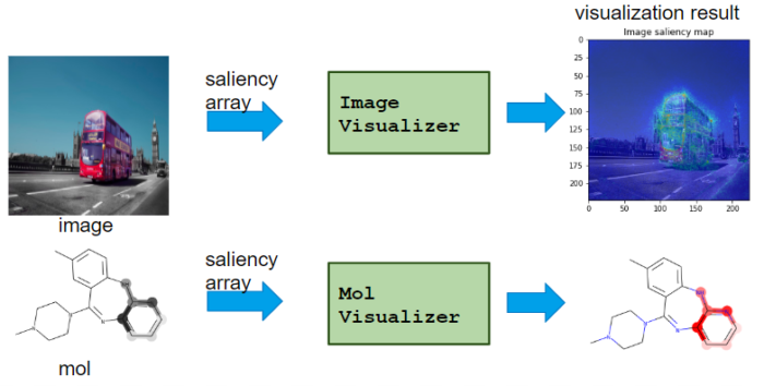
It visualizes saliency from Calcualtor class.
– TableVisualizer: plot feature importance for each table data
– ImageVisualizer: plot saliency map of image
– MolVisualizer: plot saliency map of molecule
As shown, Visualizer differs for each application.
visualize method
Visualizer plots figure with visualize method.
Note that Calculator class calcultes saliency with batch, but visualizer visualizes one data, so you need to specify it.
# Instantiation
visualizer = ImageVisualizer()

# Visualize `i`-th data
i = 0
visualizer.visualize(saliency[i])
The figure can be saved by setting save_filepath argument.
# Save saliency map
visualizer.visualize(saliency[i], save_filepath='saliency.png')
Examples
It was a long explanation,,, now let’s use it!
Table data application: calculate feature importance
Neural Network is MLP (Multi Layer Parceptron), Dataset is iris dataset provided by sklearn.
iris dataset is to classify 3 flower species ‘setosa’, ‘versicolor’, ‘virginica’, from 4 features ‘sepal length (cm)’, ‘sepal width (cm)’, ‘petal length (cm)’, ‘petal width (cm)’.
# model
from chainer.functions import relu, dropout
from chainer_chemistry.models.mlp import MLP
from chainer_chemistry.models.prediction.classifier import Classifier

def activation_relu_dropout(h):
return dropout(relu(h), ratio=0.5)

out_dim = len(iris.target_names)
predictor = MLP(out_dim=out_dim, hidden_dim=48, n_layers=2, activation=activation_relu_dropout)
classifier = Classifier(predictor)

# dataset
import sklearn
from sklearn import datasets
import numpy as np
from chainer_chemistry.datasets.numpy_tuple_dataset import NumpyTupleDataset

iris = datasets.load_iris()
# All dataset is to train for simplicity
dataset = NumpyTupleDataset(iris.data.astype(np.float32), iris.target.astype(np.int32))
train = dataset
Model’s training code is omitted (please refer the code on github). After training the model, we can use saliency module.
First, use Calculator compute -> aggregate to calculate saliency.
from chainer_chemistry.saliency.calculator.gradient_calculator import GradientCalculator

# 1. instantiation
gradient_calculator = GradientCalculator(classifier)
# 2. compute
saliency_samples_vanilla = gradient_calculator.compute(train, M=1)
# 3. aggregate
saliency_vanilla = gradient_calculator.aggregate(
saliency_samples_vanilla, ch_axis=None, method='square')
Second, use Visualizer visualize method to plot figure.
from chainer_chemistry.saliency.visualizer.table_visualizer import TableVisualizer
from chainer_chemistry.saliency.visualizer.common import normalize_scaler

visualizer = TableVisualizer()
# Visualize saliency of `i`-th data
i = 0
visualizer.visualize(saliency_vanilla[i], feature_names=iris.feature_names,
scaler=normalize_scaler)
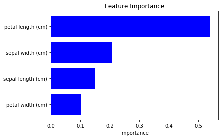
We can see how the each feature contributes to the final output prediction loss.
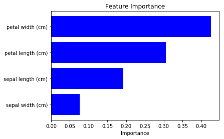
We saw saliency for 0-th data above, now we can calculate average along dataset to show feature importance for all data (which roughly corresponds to model’s feature importance).
saliency_mean = np.mean(saliency_vanilla, axis=0)
visualizer.visualize(saliency_mean, feature_names=iris.feature_names, num_visualize=-1,
scaler=normalize_scaler)
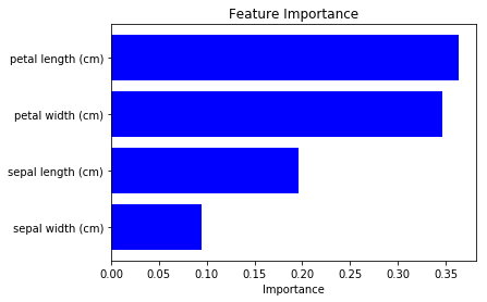
We can see “petal length” and “petal width” are more important. (note that the result differs according to the model’s training condition, be careful.)
To check above result is plausible, I tried to plot feature impotance of Random Forest from sklearn (code).
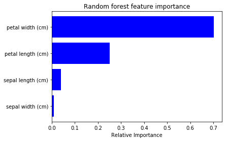
Even though the absolute importance value differs, its order is same. So I feel the saliency calculation of NN is also useful for feature selection etc 🙂
Image data: show saliency map for classification task
Training CNN takes time, so I will use pre-trained model. I will use VGG16 model provided by Chainer this time.
from chainer.links.model.vision.vgg import VGG16Layers

predictor = VGG16Layers()
It automatically download pretrained parameters, with only this code.
ImageNet correct label name is downloaded from here.
import numpy as np

with open('imagenet1000_clsid_to_human.txt') as f:
lines = f.readlines()

def extract_value(s):
quote_str = s[s.index(':') + 2]
return s[s.find(quote_str)+1:s.rfind(quote_str)]

classes = np.array([extract_value(line) for line in lines])
classes is 1000 class correct label as follows:
array(['tench, Tinca tinca', 'goldfish, Carassius auratus',
'great white shark, white shark, man-eater, man-eating shark, Carcharodon carcharias',
'tiger shark, Galeocerdo cuvieri', 'hammerhead, hammerhead shark',
'electric ray, crampfish, numbfish, torpedo', 'stingray', 'cock', ...
The images used in inference are downloaded from Pexels under CC0 license.


– Basketball image
– Bus image
– Dog image
Let’s try prediction at first.
from PIL import Image
import numpy as np

import chainer
import chainer.functions as F

# basketball, bus, dog
image_paths = ['./input/pexels-photo-945471.jpeg', './input/pexels-photo-45923.jpeg',
'./input/pexels-photo-58997.jpeg']

imgs = [Image.open(fp) for fp in image_paths]
x = xp.asarray([chainer.links.model.vision.vgg.prepare(img) for img in imgs])
with chainer.using_config('train', False):
result = predictor.forward(x, layers=['prob'])
prob = result['prob']

lables_pred = np.argsort(cuda.to_cpu(prob.array), axis=1)[:, ::-1]

for i in range(len(lables_pred)):
print('i', i, 'labels_pred', lables_pred[i, :5], classes[lables_pred[i, :5]])
`
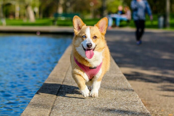
i 0 classes ['basketball' 'punching bag, punch bag, punching ball, punchball'
'rugby ball' 'barrel, cask' 'barbell']
i 1 classes ['trailer truck, tractor trailer, trucking rig, rig, articulated lorry, semi'
'passenger car, coach, carriage'
'streetcar, tram, tramcar, trolley, trolley car'
'fire engine, fire truck' 'trolleybus, trolley coach, trackless trolley']
i 2 classes ['basenji' 'Pembroke, Pembroke Welsh corgi' 'Ibizan hound, Ibizan Podenco'
'dingo, warrigal, warragal, Canis dingo' 'kelpie']
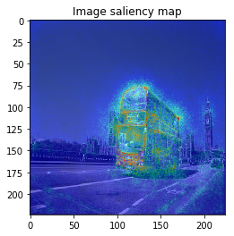
When we see the result, 1-st image is correctly predicted as Basketball, 2nd image is predicted as trailer truck though it is actually bus, 3rd image is predicted as basenji (ImageNet contains various dog’s species as label, I do not know this is indeed correct or not…).
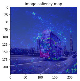
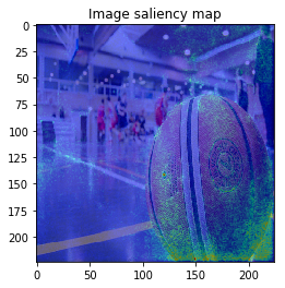
VanillaGrad
So let’s proceed to saliency calculation. This time, I will calculate saliency for “why predicting the label of top prediction”, not for the ground truth label. For example in 2nd image, we calculate saliency for why the CNN model predicted “trailer truck”, so the ground truth label (and the model predicts correct label or not) is not related.
I can set output_var as “softmax cross entropy between top prediction label” (instead of ground truth label).
import chainer.functions as F
from chainer import cuda

def eval_fun(x):
result = predictor(x, layers=['fc8'])
out = result['fc8']
xp = cuda.get_array_module(out.array)
labels_pred = xp.argmax(out.array, axis=1).astype(xp.int32)
loss = F.softmax_cross_entropy(out, labels_pred)
return loss
Once eval_fun is defined, we can follow usual step: Calculator compute -> aggregate, ImageVisualizer visualize, to see the result.
from chainer_chemistry.saliency.calculator.gradient_calculator import GradientCalculator

# 1. instantiation
gradient_calculator = GradientCalculator(predictor, eval_fun=eval_fun, device=device)
# --- VanillaGrad ---
# 2. compute
saliency_samples_vanilla = gradient_calculator.compute(x)

# 3. aggregate
saliency_vanilla = gradient_calculator.aggregate(
saliency_samples_vanilla, ch_axis=2, method='abs')

# saliency_samples (1, 3, 3, 224, 224) -> M, minibatch, ch, h, w
print('saliency_samples', saliency_samples_vanilla.shape)
# saliency (3, 224, 224) -> minibatch, h, w
print('saliency', saliency_vanilla.shape)
We set ch_axis=2 in aggregate method, this is different from usual (minibatch, ch, h, w) image shape, because sampling_axis is added in front.
ImageVisualizer visualization result is as follows:
from chainer_saliency.visualizer.image_visualizer import ImageVisualizer

visualizer = ImageVisualizer()

for index in range(len(saliency_vanilla)):
image = imgs[index].resize(saliency_vanilla[index].shape)
visualizer.visualize(saliency_vanilla[index], image, show_colorbar=False)
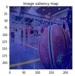
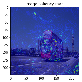
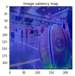
It looks the model focuses on right place,,, but it is too noisy to see the result.
SmoothGrad
Next, let’s calculate SmoothGrad. We can set noise_sampler argument in Calculator compute method.
from chainer_chemistry.saliency.calculator.common import GaussianNoiseSampler

M = 30

# --- SmoothGrad ---
# 2. compute
saliency_samples_smooth = gradient_calculator.compute(x, M=M, noise_sampler=GaussianNoiseSampler())

# 3. aggregate
saliency_smooth = gradient_calculator.aggregate(
saliency_samples_smooth, ch_axis=2, method='abs')

for index in range(len(saliency_vanilla)):
image = imgs[index].resize(saliency_smooth[index].shape)
visualizer.visualize(saliency_smooth[index], image, show_colorbar=False)
aggregate, visualize methods are same with VanillaGrad.
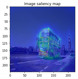
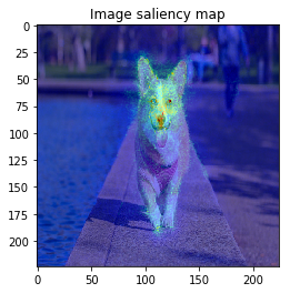
The figure looks much better, we can see model focuses on the edge of objects.
BayesGrad
At last, we will try BayesGrad. It requires that the model has stochastic operation. This time, VGG16 has dropout operation so it is applicable.
To calculate BayesGrad, we only need to set train=True in Calculator compute method. Chainer automatically enables dropout so that output is different in each samples, results that we can calculate saliency samples (gradient) for prediction distribution.
M = 30
# --- BayesGrad ---
# 2. compute
saliency_samples_bayes = gradient_calculator.compute(x, M=M, train=True)
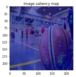
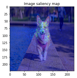
This time, the result is similar to VanillaGrad.
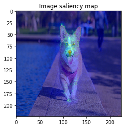
When I try combining both SmoothGrad & BayesGrad, the result are as follows:

Molecule data: plot property contribution map for regression task
For regression task, we can calculate saliency to consider its sign, to show that the input contributes to positive or negative to the prediction.
In this last example, I will use Graph convolution model in Chainer Chemistry, to visualize water solubility contribution for each atom.
ESOL dataset is used for water solubility dataset.
import numpy as np
import chainer
from chainer.functions import relu, dropout

from chainer_chemistry.models.ggnn import GGNN
from chainer_chemistry.datasets.numpy_tuple_dataset import NumpyTupleDataset
from chainer_chemistry.datasets.zinc import get_zinc250k
from chainer_chemistry.dataset.preprocessors.ggnn_preprocessor import GGNNPreprocessor
from chainer_chemistry.models.mlp import MLP
from chainer_chemistry.models.prediction.regressor import Regressor


# Model
def activation_relu_dropout(h):
    return dropout(relu(h), ratio=0.25)

class GraphConvPredictor(chainer.Chain):
    def __init__(self, graph_conv, mlp=None):
        """Initializes the graph convolution predictor.
        Args:
            graph_conv: The graph convolution network required to obtain
                        molecule feature representation.
            mlp: Multi layer perceptron; used as the final fully connected
                 layer. Set it to `None` if no operation is necessary
                 after the `graph_conv` calculation.
        """
        super(GraphConvPredictor, self).__init__()
        with self.init_scope():
            self.graph_conv = graph_conv
            if isinstance(mlp, chainer.Link):
                self.mlp = mlp
        if not isinstance(mlp, chainer.Link):
            self.mlp = mlp

    def __call__(self, atoms, adjs):
        x = self.graph_conv(atoms, adjs)
        if self.mlp:
            x = self.mlp(x)
        return x

n_unit = 32
conv_layers = 4
class_num = 1
device = 0  # -1 for CPU

ggnn = GGNN(out_dim=n_unit, hidden_dim=n_unit, n_layers=conv_layers)
mlp = MLP(out_dim=class_num, hidden_dim=n_unit, activation=activation_relu_dropout)
predictor = GraphConvPredictor(ggnn, mlp)
regressor = Regressor(predictor, device=device)

# Dataset
preprocessor = GGNNPreprocessor()

result = get_molnet_dataset('delaney', preprocessor, labels=None, return_smiles=True)
train = result['dataset'][0]
smiles = result['smiles'][0]
After training the model (see repository for the code), we can proceed to visualization.
This time, we want to focus on contribution to the output prediction instead of loss. So we can define eval_fun to set output_var as predictor‘s output.
Also, we need to take care that input x is label of the node, gradient is not propagated until this input, we need to adopt gradient of the variable after embed layer, which is hidden layer’s variable.
In this kind of case, to set target_var as intermediate variable in the model, we can use VariableMonitorLinkHook.
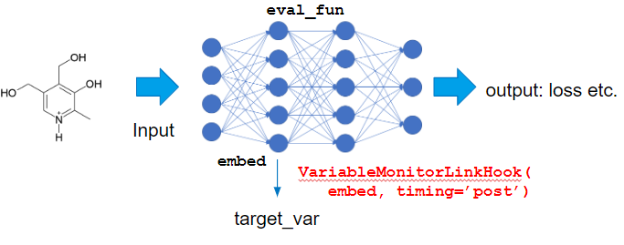
I use IntegratedGradientsCalculator this time, to calculate saliency:
import chainer.functions as F

from chainer_chemistry.saliency.calculator.gradient_calculator import GradientCalculator
from chainer_chemistry.saliency.calculator.integrated_gradients_calculator import IntegratedGradientsCalculator
from chainer_chemistry.link_hooks.variable_monitor_link_hook import VariableMonitorLinkHook


def eval_fun(x, adj, t):
    pred = predictor(x, adj)
    pred_summed = F.sum(pred)
    return pred_summed

# 1. instantiation
calculator = IntegratedGradientsCalculator(
predictor, steps=5, eval_fun=eval_fun, target_extractor=VariableMonitorLinkHook(ggnn.embed, timing='post'),
device=device)
Visualization results are as follows,
from chainer_chemistry.saliency.visualizer.mol_visualizer import SmilesVisualizer
from chainer_chemistry.saliency.visualizer.common import abs_max_scaler

visualizer = SmilesVisualizer()
# 2. compute
saliency_samples_vanilla = calculator.compute(
train, M=1, converter=concat_mols)
method = 'raw'
saliency_vanilla = calculator.aggregate(
saliency_samples_vanilla, ch_axis=3, method=method)
i = 153
visualizer.visualize(saliency_vanilla[i], smiles[i])
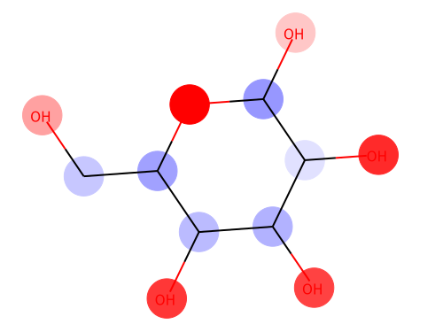
Red color shows the positive effect on solubility (Hydrophilic), blue color shows the negative effect on solubility (Hydrophobic).
Above figure matches the common sense of Hydrophilic effects usually occurs at polarization exists (OH), and we can see Hydrophobic effects where C-chain continues.
Conclusion
I introduced saliency module, which is highly flexible and applicable to any domain.
You can try all the examples with few machine resources, only with CPU, so please try!! (Saliency map visualization of image uses pre-trained model so only inference is necessary).