Source code is uploaded on github.
The sample image is obtained from PEXELS.
What is the difference between convolutional layer and linear layer? What kind of intuition is in behind of using convolutional layer in deep neural network?
This hands on shows some effects by convolutional layer to provide some intution about what convolutional layer do.
import os

import numpy as np
import matplotlib.pyplot as plt
import cv2

%matplotlib inline

basedir = './src/cnn/images'


def read_rgb_image(imagepath):
    image = cv2.imread(imagepath)  # Height, Width, Channel
    (major, minor, _) = cv2.__version__.split(".")
    if major == '3':
        # version 3 is used, need to convert
        image = cv2.cvtColor(image, cv2.COLOR_BGR2RGB)
    else:
        # Version 2 is used, not necessary to convert
        pass
    return image


def read_gray_image(imagepath):
    image = cv2.imread(imagepath)  # Height, Width, Channel
    (major, minor, _) = cv2.__version__.split(".")
    if major == '3':
        # version 3 is used, need to convert
        image = cv2.cvtColor(image, cv2.COLOR_BGR2GRAY)
    else:
        # Version 2 is used, not necessary to convert
        image = cv2.cvtColor(image, cv2.COLOR_RGB2GRAY)
    return image


def plot_channels(array, filepath='out.jpg'):
    """Plot each channel component separately

    Args:
        array (numpy.ndarray): 3-D array (width, height, channel)

    """
    ch_number = array.shape[2]

    fig, axes = plt.subplots(1, ch_number)
    for i in range(ch_number):
        # Save each image
        # cv2.imwrite(os.path.join(basedir, 'output_conv1_{}.jpg'.format(i)), array[:, :, i])
        axes[i].set_title('Channel {}'.format(i))
        axes[i].axis('off')
        axes[i].imshow(array[:, :, i], cmap='gray')

    plt.savefig(filepath)
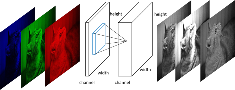
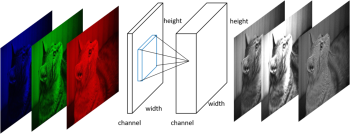
Above type of diagram often appears in Convolutional neural network field. Below figure explains its notation.
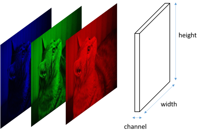
Cuboid represents the “image” array where this image might not mean the meaningful picture. Horizontal axis represents channel number, vertical axis for image height and depth axis for image width respectively.
Contents
Convolution layer – basic usage
Input format of convolutional layer is in the order, (batch index, channel, height, width). Since openCV image format is in the order (height, width, channel), this dimension order need to be converted to input to convolution layer.
It can be done by using transpose method.
L.Convolution2D(in_channels, out_channels, ksize)
in_channels: input channel number.out_channels: output channel number.ksize: kernel size.
also, following parameters is often set
pad: paddingstride: stride
To understand the behavior of convolution layer, I recommend to see the animation on conv_arithmetic.
import chainer.links as L

# Read image from file, save image with matplotlib using `imshow` function
imagepath = os.path.join(basedir, 'sample.jpeg')

image = read_rgb_image(imagepath)

# height and width shows pixel size of this image
# Channel=3 indicates the RGB channel
print('image.shape (Height, Width, Channel) = ', image.shape)

conv1 = L.Convolution2D(None, 3, 5)

# Need to input image of the form (batch index, channel, height, width)
image = image.transpose(2, 0, 1)
image = image[np.newaxis, :, :, :]

# Convert from int to float
image = image.astype(np.float32)
print('image shape', image.shape)
out_image = conv1(image).data
print('shape', out_image.shape)
out_image = out_image[0].transpose(1, 2, 0)
print('shape 2', out_image.shape)
plot_channels(out_image,
              filepath=os.path.join(basedir, 'output_conv1.jpg'))

#plt.imshow(image)
#plt.savefig('./src/cnn/images/out.jpg')
image.shape (Height, Width, Channel) = (380, 512, 3)image shape (1, 3, 380, 512)shape (1, 3, 376, 508)shape 2 (376, 508, 3)
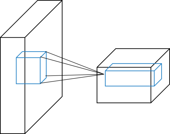
Convolution2D layer takes 4-dim array as input and outputs 4-dim array. Graphical meaning of this input-output relation ship is drawn in below figure.
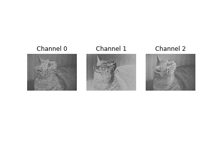
When the in_channels is set to None, its size is determined at the first time when it is used. i.e., out_image = conv1(image).data in above code.
The internal parameter W is initialized randomly at that time. As you can see, output_conv1.jpg shows the result after random filter is applied.
Some “feature” can be extracted by applying convolution layer.
For example, random fileter sometimes acts as “blurring” or “edge extracting” image.
To understand the intuitive meaning of convolutional layer in more detail, please see below example.
gray_image = read_gray_image(imagepath)
print('gray_image.shape (Height, Width) = ', gray_image.shape)

# Need to input image of the form (batch index, channel, height, width)
gray_image = gray_image[np.newaxis, np.newaxis, :, :]
# Convert from int to float
gray_image = gray_image.astype(np.float32)

conv_vertical = L.Convolution2D(1, 1, 3)
conv_horizontal = L.Convolution2D(1, 1, 3)

print(conv_vertical.W.data)
conv_vertical.W.data = np.asarray([[[[-1., 0, 1], [-1, 0, 1], [-1, 0, 1]]]])
conv_horizontal.W.data = np.asarray([[[[-1., -1, -1], [0, 0., 0], [1, 1, 1]]]])

print('image.shape', image.shape)
out_image_v = conv_vertical(gray_image).data
out_image_h = conv_horizontal(gray_image).data
print('out_image_v.shape', out_image_v.shape)
out_image_v = out_image_v[0].transpose(1, 2, 0)
out_image_h = out_image_h[0].transpose(1, 2, 0)
print('out_image_v.shape (after transpose)', out_image_v.shape)

cv2.imwrite(os.path.join(basedir, 'output_conv_vertical.jpg'), out_image_v[:, :, 0])
cv2.imwrite(os.path.join(basedir, 'output_conv_horizontal.jpg'), out_image_h[:, :, 0])
gray_image.shape (Height, Width) = (380, 512)[[[[-0.17837302 0.2948513 -0.0661072 ] [ 0.02076577 -0.14251317 -0.05151904] [ 0.01675515 0.07612066 0.37937522]]]]image.shape (1, 3, 380, 512)out_image_v.shape (1, 1, 378, 510)out_image_v.shape (after transpose) (378, 510, 1)
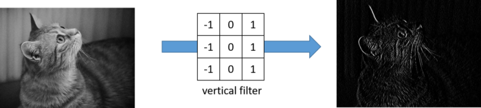
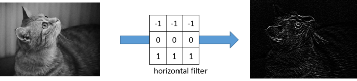
As you can see from the result, each convolution layer acts as emphasizing/extracting the color difference along specific direction. In this way “filter”, also called “kernel” can be considered as feature extractor.
Convolution with stride
The default value of stride is 1. If this value is specified, convolution layer will reduce output image size.
Practically, stride=2 is often used to generate the output image of the height & width almost half of the input image.
print('image.shape (Height, Width, Channel) = ', image.shape)
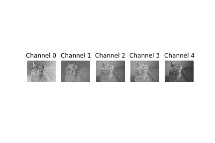
conv2 = L.Convolution2D(None, 5, 3, 2)
print('input image.shape', image.shape)
out_image = conv2(conv1(image)).data
print('out_image.shape', out_image.shape)
out_image = out_image[0].transpose(1, 2, 0)
plot_channels(out_image,
filepath=os.path.join(basedir, 'output_conv2.jpg'))
image.shape (Height, Width, Channel) = (1, 3, 380, 512)input image.shape (1, 3, 380, 512)out_image.shape (1, 5, 187, 253)
As written in the Chainer docs, the input and output shape relation is given in below formula:
$$ w_O = (w_I + 2w_P – w_K) / s_X + 1 $$where each symbol means that
- \(h\): height
- \(w\): width
- \(I\): input
- \(O\): output
- \(P\): padding
- \(K\): kernel size
Max pooling
Convolution layer with stride can be used to look wide range feature, another popular method is to use max pooling.
Max pooling function extracts the maximum value in the kernel, and it dispose the rest pixel’s information.
This behavior is beneficial to impose translational symmetry. For example, consider the dog’s picture. Even if the each pixel shifted one pixel, is should be still recognized as dog. So translational symmetry can be exploited to reduce model’s calculation time and number of internal parameters for image classification task.
from chainer import functions as F
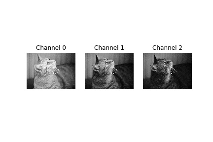
print('image.shape (Height, Width, Channel) = ', image.shape)
print('input image.shape', image.shape)
out_image = F.max_pooling_2d(image, 2).data
print('out_image.shape', out_image.shape)
out_image = out_image[0].transpose(1, 2, 0)
plot_channels(out_image,
filepath=os.path.join(basedir, 'output_max_pooling.jpg'))
image.shape (Height, Width, Channel) = (1, 3, 380, 512)input image.shape (1, 3, 380, 512)out_image.shape (1, 3, 190, 256)
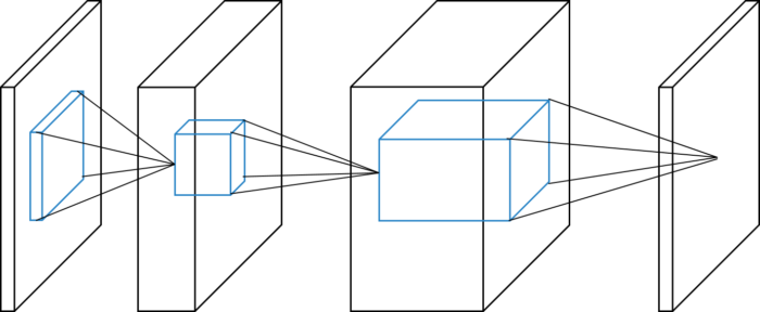
Convolutional neural network
By combining above functions with non-linear activation units, Convolutional Neural Network (CNN) can be constructed.
For non-linear activation, relu, leaky_relu, sigmoid or tanh are often used.
class SimpleCNN(chainer.Chain):
def __init__(self):
super().__init__(
conv1=L.Convolution2D(None, 5, 3),
conv2=L.Convolution2D(None, 5, 3),
)
def __call__(self, x):
h = F.relu(conv1(x))
h = F.max_pooling_2d(h, 2)
h = F.relu(conv2(h))
h = F.max_pooling_2d(h, 2)
return h
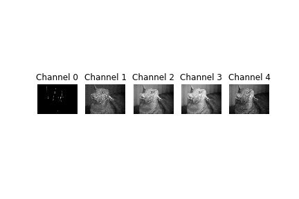
model = SimpleCNN()
print('input image.shape', image.shape)
out_image = model(image).data
print('out_image.shape', out_image.shape)
out_image = out_image[0].transpose(1, 2, 0)
plot_channels(out_image,
filepath=os.path.join(basedir, 'output_simple_cnn.jpg'))
input image.shape (1, 3, 380, 512)out_image.shape (1, 5, 47, 63)
Let’s see how this CNN can be used for image classification in the following. Before that, next post explains CIFAR-10, CIFAR-100 dataset which are famous image classification dataset for research.