2 Chain classes, “Predictor” and “Classifier” are used for this framework.
Training phase: Predictor’s output is fed into Classifier to calculate loss.
Predict/Inference phase: Only predictor’s output is used.
Predictor
Predictor simply calculates output based on input.
# Network definition Chainer v2
# 1. `init_scope()` is used to initialize links for IDE friendly design.
# 2. input size of Linear layer can be omitted
class MLP(chainer.Chain):

    def __init__(self, n_units, n_out):
        super(MLP, self).__init__()
        with self.init_scope():
            # input size of each layer will be inferred when omitted
            self.l1 = L.Linear(n_units)  # n_in -> n_units
            self.l2 = L.Linear(n_units)  # n_units -> n_units
            self.l3 = L.Linear(n_out)    # n_units -> n_out

    def __call__(self, x):
        h1 = F.relu(self.l1(x))
        h2 = F.relu(self.l2(h1))
        return self.l3(h2)
model = mlp.MLP(args.unit, 10)
Classifier
Classifier “wraps” predictors output y to calculate loss between y and actual target t.
classifier_model = L.Classifier(model)
optimizer.update(classifier_model, x, t)
which invokes classifier_model(x, t) internally, calculates loss and update internal parameter by back propagation.
Both the loss calculation in train phase and predict code for inference phase are implemented within one model, and the behavior is managed by “train flag” (or “test flag”/”predict flag”).
# Network definition
class MLP(chainer.Chain):

    def __init__(self, n_units, n_out):
        super(MLP, self).__init__()
        with self.init_scope():
            self.l1 = L.Linear(None, n_units)  # n_in -> n_units
            self.l2 = L.Linear(None, n_units)  # n_units -> n_units
            self.l3 = L.Linear(None, n_out)  # n_units -> n_out

        # Define train flag
        self.train = True

    def __call__(self, x, t=None):
        h1 = F.relu(self.l1(x))
        h2 = F.relu(self.l2(h1))
        y = self.l3(h2)
        if self.train:
            # return loss in training phase
            #y = self.predictor(x)
            self.loss = F.softmax_cross_entropy(y, t)
            self.accuracy = F.accuracy(y, t)
            return self.loss
        else:
            # return y in predict/inference phase
            return y
As default, self.train = True, and this model will calculate loss so that optimizer can update its internal parameters.
To predict value, we can set train flag to False,
model.train = False
y = model(x)
# model.train = True  # if necessary
Comparison
Predictor – Classifier framework has an advantage that Classifier module can be independent and it will be reusable. However, if loss calculation is complicated, it is difficult to apply this framework.
In train flag framework, train loss calculation and predict calculation can be independent. You can implement any loss calculation, even the loss calculation is very different from predict calculation.
Basically, you can use Predictor – Classifier framework if the loss function is typical. Use train flag framework otherwise.
argparse is used to provide configurable script code. User can pass variable when executing the code.
Below code is added to the training code
import argparse


def main():
    parser = argparse.ArgumentParser(description='Chainer example: MNIST')
    parser.add_argument('--initmodel', '-m', default='',
                        help='Initialize the model from given file')
    parser.add_argument('--batchsize', '-b', type=int, default=100,
                        help='Number of images in each mini-batch')
    parser.add_argument('--epoch', '-e', type=int, default=20,
                        help='Number of sweeps over the dataset to train')
    parser.add_argument('--gpu', '-g', type=int, default=-1,
                        help='GPU ID (negative value indicates CPU)')
    parser.add_argument('--out', '-o', default='result/2',
                        help='Directory to output the result')
    parser.add_argument('--resume', '-r', default='',
                        help='Resume the training from snapshot')
    parser.add_argument('--unit', '-u', type=int, default=50,
                        help='Number of units')
    args = parser.parse_args()

    ...
Then, these variables are configurable when executing the code from console. And these variables can be accessed by args.xxx (e.g. args.batchsize, args.epoch etc.).
You can also see what command is available using --help command or simply -h.
xxx:~/workspace/pycharm/chainer-hands-on-tutorial/src/mnist$ python train_mnist_2_predictor_classifier.py -h
usage: train_mnist_2_predictor_classifier.py [-h] [--initmodel INITMODEL]
                                             [--batchsize BATCHSIZE]
                                             [--epoch EPOCH] [--gpu GPU]
                                             [--out OUT] [--resume RESUME]
                                             [--unit UNIT]

Chainer example: MNIST

optional arguments:
  -h, --help            show this help message and exit
  --initmodel INITMODEL, -m INITMODEL
                        Initialize the model from given file
  --batchsize BATCHSIZE, -b BATCHSIZE
                        Number of images in each mini-batch
  --epoch EPOCH, -e EPOCH
                        Number of sweeps over the dataset to train
  --gpu GPU, -g GPU     GPU ID (negative value indicates CPU)
  --out OUT, -o OUT     Directory to output the result
  --resume RESUME, -r RESUME
                        Resume the training from snapshot
  --unit UNIT, -u UNIT  Number
Save and load the model or optimizer can be done using serializers, below code is to save the training result. The directory to save the result can be configured by -o option.
    parser.add_argument('--out', '-o', default='result/2',
                        help='Directory to output the result')

    ...

    # Save the model and the optimizer
    print('save the model')
    serializers.save_npz('{}/classifier.model'.format(args.out), classifier_model)
    serializers.save_npz('{}/mlp.model'.format(args.out), model)
    print('save the optimizer')
    serializers.save_npz('{}/mlp.state'.format(args.out), optimizer)
If you want to resume the training based on the previous training result, load the model and optimizer before start training.
Optimizer also owns internal parameters and thus need to be loaded for resuming training. For example, Adam holds the “first moment” m and “second moment” v explained in adam.
    parser.add_argument('--initmodel', '-m', default='',
                        help='Initialize the model from given file')
    parser.add_argument('--resume', '-r', default='',
                        help='Resume the training from snapshot')
    ...

    # Init/Resume
    if args.initmodel:
        print('Load model from', args.initmodel)
        serializers.load_npz(args.initmodel, classifier_model)
    if args.resume:
        print('Load optimizer state from', args.resume)
        serializers.load_npz(args.resume, optimizer)
[hands on] Check resume the code after first training, by running
xxx:~/workspace/pycharm/chainer-hands-on-tutorial/src/mnist$ python train_mnist_2_predictor_classifier.py -m result/2/classifier.model -r result/2/mlp.state
GPU: -1
# unit: 50
# Minibatch-size: 100
# epoch: 20

Load model from result/2/classifier.model
Load optimizer state from result/2/mlp.state
epoch 1
graph generated
train mean loss=0.037441188701771655, accuracy=0.9890166732668877, throughput=57888.5195400998 images/sec
test  mean loss=0.1542429528321469, accuracy=0.974500007033348
You can check pre-trained model is used and accuracy is high (98%) from the beginning.
Note that these codes are not executed if no configuration is specified, model and optimizer is not loaded and default initial value is used.
Classifier
Build-in Link, L.Classifier is used instead of custom class SoftmaxClassifier in train_mnist_1_minimum.py.
classifier_model = L.Classifier(model)
I implemented SoftmaxClassifier, to let you understand the loss calculation (suing softmax for classification task). However, most of the classification task use this function and it is already supported as a build-in Link L.Classifier.
You can consider using L.Classifier when coding a classification task.
You already studied basics of Chainer and MNIST dataset. Now we can proceed to the MNIST classification task. We want to create a classifier that classifies MNIST handwritten image into its digit. In other words, classifier will get array which represents MNIST image as input and outputs its label.
※ Chainer contains modules called Trainer, Iterator, Updater, which makes your training code more organized. It is quite nice to write your training code by using them in higher level syntax. However, its abstraction makes difficult to understand what is going on during the training. For those who want to learn deep learning in more detail, I think it is nice to know “primitive way” of writing training code. Therefore, I intentionally don’t to use these modules at first to explain training code.
[hands on] Before going to read the explanation, try to execute train_mnist_1_minimum.py. If you are using IDE like pycharm, just press run button. If you are going to run from command line, go to src directory first and execute
python mnist/train_mnist_1_minimum.py
You can see the log like below, indicating that the loss in decreasing through the training and accuracy is increasing.
GPU: -1 # unit: 50 # Minibatch-size: 100 # epoch: 20 out directory: result/1_minimum epoch 1 train mean loss=0.41262895802656807, accuracy=0.8860333333909511, throughput=54883.71423542936 images/sec test mean loss=0.21496000131592155, accuracy=0.9357000035047531 epoch 2 train mean loss=0.1967763691022992, accuracy=0.942733335296313, throughput=66559.17396858479 images/sec test mean loss=0.17020921929739416, accuracy=0.9499000030755996 epoch 3 train mean loss=0.1490274258516729, accuracy=0.9558166695634523, throughput=66375.93210754421 images/sec test mean loss=0.1352944350033067, accuracy=0.9595000040531159 ...
Of course, it is ok that you may not understand the meaning of this log here. I will explain the detail one by one in the following.
Define Network and loss function
Let’s adopt Multi Layer Perceptron (MLP), which is a most simple neural network, as our model. This is written as follows with Chainer,
class MLP(chainer.Chain):
    """Neural Network definition, Multi Layer Perceptron"""
    def __init__(self, n_units, n_out):
        super(MLP, self).__init__()
        with self.init_scope():
            # the size of the inputs to each layer will be inferred when `None`
            self.l1 = L.Linear(None, n_units)  # n_in -> n_units
            self.l2 = L.Linear(None, n_units)  # n_units -> n_units
            self.l3 = L.Linear(None, n_out)    # n_units -> n_out

    def __call__(self, x):
        h1 = F.relu(self.l1(x))
        h2 = F.relu(self.l2(h1))
        y = self.l3(h2)
        return y
[Memo] In chainer v1, it was written as follows,
# Neural Network definition, Multi Layer Perceptron
class MLP(chainer.Chain):

    def __init__(self, n_units, n_out):
        super(MLP, self).__init__(
            # the size of the inputs to each layer will be inferred
            l1=L.Linear(None, n_units),  # n_in -> n_units
            l2=L.Linear(None, n_units),  # n_units -> n_units
            l3=L.Linear(None, n_out),  # n_units -> n_out
        )

    def __call__(self, x):
        h1 = F.relu(self.l1(x))
        h2 = F.relu(self.l2(h1))
        y = self.l3(h2)
        return y
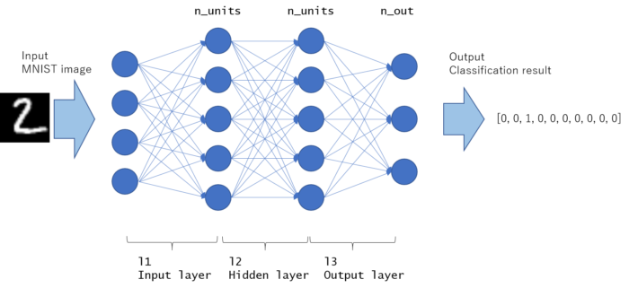
This model is graphically drawn as follows. All nodes are fully connected, and the network with this kinds of structure is called MLP (Multi layer perceptron).
The fast part is input layer and the last part is output layer. The rest middle part of the layer is called “hidden layer”. This example contains only 1 hidden layer, but hidden layers may exist more than 1 in general (If you construct the network deeper, the number of hidden layer increases).
MLP (Multi Layer Perceptron)
As written in __call__ function, it will take x (array indicating image) as input and return y (indicating predicted probability for each label) as output.
However, this is not enough for training the model. We need loss function to be optimized. In classification task, softmax cross entropy loss is often used.
Output of Linear layer can take arbitrary real number, Softmax function converts it into between 0-1, thus we can consider it as “probability for this label”. Cross entropy is to calculate loss between two probability distributions. Chainer has utility function F.softmax_cross_entropy(y, t) to calculate softmax of y followed by cross entropy with t. Loss will be smaller if the probability distribution predicted as y is equal to the actual probability distribution t. Intuitively, loss decreases when model can predict correct label given image.
Here I will skip more detail explanation, please study by yourself. Here is some reference,
    unit = 50  # Number of hidden layer units
    ...
    # Set up a neural network to train
    model = MLP(unit, 10)
    # Classifier will calculate classification loss, based on the output of model
    classifier_model = SoftmaxClassifier(model)
First, MLP model is created. n_out is set to 10 because MNIST has 10 patterns, from 0 until 9, in label. Then classifier_model is created based on the MLP model as its predictor. As you can see here, Network of Chain class can be “chained” to construct new network which is also Chain class. I guess this is the reason the name “Chainer” comes from.
Once loss function calculation is defined in __call__ function of model, you can set this model into Optimizer to proceed training.
    # Setup an optimizer
    optimizer = chainer.optimizers.Adam()
    optimizer.setup(classifier_model)
            # Pass the loss function (Classifier defines it) and its arguments
            optimizer.update(classifier_model, x, t)
This code will calculate the loss as classifier_model(x, t) and tune (optimize) internal paramaters of model with Optimizer’s algorithm (Adam in this case).
Note that Back propagation is done automatically inside this update code, so you don’t need to write these codes explicitly.
As explain below, we will pass x and t in minibatch unit.
Use GPU
Chainer support GPU for calculation speed-up. To use GPU, PC must have NVIDIA GPU and you need to install CUDA, and better to install cudnn followed by installing chainer.
To write GPU compatible code, just add these 3 lines.
    if gpu >= 0:
        chainer.cuda.get_device(gpu).use()  # Make a specified GPU current
        classifier_model.to_gpu()           # Copy the model to the GPU
    xp = np if gpu < 0 else cuda.cupy
You need to set gpu device id in variable gpu.
If you don’t use gpu, set gpu=-1, which indicates not to use GPU and only use CPU. In that case numpy (written as np in above) is used for array calculation.
If you want to use gpu, set gpu=0 etc (usual consumer PC with NVIDIA GPU contains one GPU core, thus only gpu device id=0 can be used. GPU cluster have several GPUs (0, 1, 2, 3 etc) in one PC). In this case, call chainer.cuda.get_device(gpu).use() for specifying which GPU device to be used and model.to_gpu() to copy model’s internal parameters into GPU. In this case cupy is used for array calculation.
cupy
In python science calculation, numpy is widely used for vector, matrix and general tensor calculation. numpy will optimize these linear calculation with CPU automatically. cupy can be considered as GPU version of numpy, so that you can write GPU calculation code almost same with numpy. cupy is developed by Chainer team, as chainer.cuda.cupy in Chainer version 1.
However, cupy itself can be used as GPU version of numpy, thus applicable to more wide use case, not only for chainer. So cupy will be independent from chainer, and provided as cupy module from Chainer version 2.
GPU performance
How much different if GPU can be used? Below table show the image throughput with the model’s hidden layer unit size
unit
CPU: Intel Core i7-6700 K Quad-core 4GHz
GPU: NVIDIA 980 Ti 2816 CUDA core 1 GHz base clock
How many times faster?
1000
5500
38000
×6.9
3000
700
13000
×18.6
When the neural network size is large, many calculation can be parallelized and GPU advantage affect more. In some cases, GPU is about 20 times faster than CPU.
[Hands on] If you have NVIDIA GPU, compare the performance between CPU & GPU in your environment.
Train and Evaluation (Test)
train_mnist_1_minimum.py consists of 2 phase, training phase and evaluation (test) phase.
In regression/classification task in machine learning, you need to verify the model’s generalization performance. Even loss is decreasing with training dataset, it is not always true that loss for test (unseen) dataset is small.
Especially, we should take care overfitting problem. To cooperate this, you can check test dataset loss also decreases through the training.
Training phase
optimizer.update code will update model’s internal parameter to decrease loss.
Random permutation is to get random sample for constructing minibatch.
If training loss is not decreasing from the beginning, the root cause may be bug or some hyper parameter setting is wrong. When training loss stops decreasing (saturated), it is ok to stop the training.
        # training
        perm = np.random.permutation(N)
        sum_accuracy = 0
        sum_loss = 0
        start = time.time()
        for i in six.moves.range(0, N, batchsize):
            x = chainer.Variable(xp.asarray(train[perm[i:i + batchsize]][0]))
            t = chainer.Variable(xp.asarray(train[perm[i:i + batchsize]][1]))

            # Pass the loss function (Classifier defines it) and its arguments
            optimizer.update(classifier_model, x, t)

            sum_loss += float(classifier_model.loss.data) * len(t.data)
            sum_accuracy += float(classifier_model.accuracy.data) * len(t.data)
        end = time.time()
        elapsed_time = end - start
        throughput = N / elapsed_time
        print('train mean loss={}, accuracy={}, throughput={} images/sec'.format(
            sum_loss / N, sum_accuracy / N, throughput))
Evaluation (test) phase
We must not call optimizer.update code. Test dataset is considered as unseen data for model. Should not be included as training information.
We don’t need to take random permutation in test phase, only sum_loss and sum_accuracy is necessary.
Evaluation code does (should have) no affect to model. This is just to check loss for test dataset. Ideal pattern is of course test loss decreases through the training.
        # evaluation
        sum_accuracy = 0
        sum_loss = 0
        for i in six.moves.range(0, N_test, batchsize):
            index = np.asarray(list(range(i, i + batchsize)))
            x = chainer.Variable(xp.asarray(test[index][0]))
            t = chainer.Variable(xp.asarray(test[index][1]))

            loss = classifier_model(x, t)
            sum_loss += float(loss.data) * len(t.data)
            sum_accuracy += float(classifier_model.accuracy.data) * len(t.data)

        print('test  mean loss={}, accuracy={}'.format(
            sum_loss / N_test, sum_accuracy / N_test))
1234567891011121314
# evaluation sum_accuracy = 0 sum_loss = 0 for i in six.moves.range(0, N_test, batchsize): index = np.asarray(list(range(i, i + batchsize))) x = chainer.Variable(xp.asarray(test[index][0])) t = chainer.Variable(xp.asarray(test[index][1])) loss = classifier_model(x, t) sum_loss += float(loss.data) * len(t.data) sum_accuracy += float(classifier_model.accuracy.data) * len(t.data) print(‘test mean loss={}, accuracy={}’.format( sum_loss / N_test, sum_accuracy / N_test))
If this test loss is not decreasing while training loss is decreasing, it is a sign that model is overfitting. Then, you need to take action
Increase the data size (if possible). – Data augmentation is one method to increase the data effectively.
Decrease the number of internal parameters in neural network – Try more simple network
Add Regularization term
Put all codes together,
"""
Very simple implementation for MNIST training code with Chainer using
Multi Layer Perceptron (MLP) model

This code is to explain the basic of training procedure.

"""
from __future__ import print_function
import time
import os
import numpy as np
import six

import chainer
import chainer.functions as F
import chainer.links as L
from chainer import cuda
from chainer import serializers


class MLP(chainer.Chain):
    """Neural Network definition, Multi Layer Perceptron"""
    def __init__(self, n_units, n_out):
        super(MLP, self).__init__(
            # the size of the inputs to each layer will be inferred
            l1=L.Linear(None, n_units),  # n_in -> n_units
            l2=L.Linear(None, n_units),  # n_units -> n_units
            l3=L.Linear(None, n_out),  # n_units -> n_out
        )

    def __call__(self, x):
        h1 = F.relu(self.l1(x))
        h2 = F.relu(self.l2(h1))
        y = self.l3(h2)
        return y


class SoftmaxClassifier(chainer.Chain):
    """Classifier is for calculating loss, from predictor's output.
    predictor is a model that predicts the probability of each label.
    """
    def __init__(self, predictor):
        super(SoftmaxClassifier, self).__init__(
            predictor=predictor
        )

    def __call__(self, x, t):
        y = self.predictor(x)
        self.loss = F.softmax_cross_entropy(y, t)
        self.accuracy = F.accuracy(y, t)
        return self.loss


def main():
    # Configuration setting
    gpu = -1                  # GPU ID to be used for calculation. -1 indicates to use only CPU.
    batchsize = 100           # Minibatch size for training
    epoch = 20                # Number of training epoch
    out = 'result/1_minimum'  # Directory to save the results
    unit = 50                 # Number of hidden layer units, try incresing this value and see if how accuracy changes.

    print('GPU: {}'.format(gpu))
    print('# unit: {}'.format(unit))
    print('# Minibatch-size: {}'.format(batchsize))
    print('# epoch: {}'.format(epoch))
    print('out directory: {}'.format(out))

    # Set up a neural network to train
    model = MLP(unit, 10)
    # Classifier will calculate classification loss, based on the output of model
    classifier_model = SoftmaxClassifier(model)

    if gpu >= 0:
        chainer.cuda.get_device(gpu).use()  # Make a specified GPU current
        classifier_model.to_gpu()           # Copy the model to the GPU
    xp = np if gpu < 0 else cuda.cupy

    # Setup an optimizer
    optimizer = chainer.optimizers.Adam()
    optimizer.setup(classifier_model)

    # Load the MNIST dataset
    train, test = chainer.datasets.get_mnist()

    n_epoch = epoch
    N = len(train)       # training data size
    N_test = len(test)  # test data size

    # Learning loop
    for epoch in range(1, n_epoch + 1):
        print('epoch', epoch)

        # training
        perm = np.random.permutation(N)
        sum_accuracy = 0
        sum_loss = 0
        start = time.time()
        for i in six.moves.range(0, N, batchsize):
            x = chainer.Variable(xp.asarray(train[perm[i:i + batchsize]][0]))
            t = chainer.Variable(xp.asarray(train[perm[i:i + batchsize]][1]))

            # Pass the loss function (Classifier defines it) and its arguments
            optimizer.update(classifier_model, x, t)

            sum_loss += float(classifier_model.loss.data) * len(t.data)
            sum_accuracy += float(classifier_model.accuracy.data) * len(t.data)
        end = time.time()
        elapsed_time = end - start
        throughput = N / elapsed_time
        print('train mean loss={}, accuracy={}, throughput={} images/sec'.format(
            sum_loss / N, sum_accuracy / N, throughput))

        # evaluation
        sum_accuracy = 0
        sum_loss = 0
        for i in six.moves.range(0, N_test, batchsize):
            index = np.asarray(list(range(i, i + batchsize)))
            x = chainer.Variable(xp.asarray(test[index][0]))
            t = chainer.Variable(xp.asarray(test[index][1]))

            loss = classifier_model(x, t)
            sum_loss += float(loss.data) * len(t.data)
            sum_accuracy += float(classifier_model.accuracy.data) * len(t.data)

        print('test  mean loss={}, accuracy={}'.format(
            sum_loss / N_test, sum_accuracy / N_test))

    # Save the model and the optimizer
    if not os.path.exists(out):
        os.makedirs(out)
    print('save the model')
    serializers.save_npz('{}/classifier_mlp.model'.format(out), classifier_model)
    serializers.save_npz('{}/mlp.model'.format(out), model)
    print('save the optimizer')
    serializers.save_npz('{}/mlp.state'.format(out), optimizer)

if __name__ == '__main__':
    main()
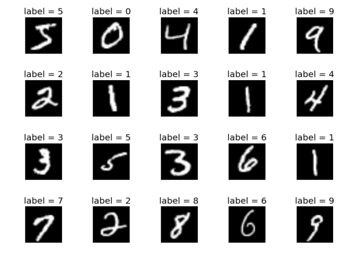
The dataset consists of pair, “handwritten digit image” and “label”. Digit ranges from 0 to 9, meaning 10 patterns in total.
handwritten digit image: This is gray scale image with size 28 x 28 pixel.
label : This is actual digit number this handwritten digit image represents. It is either 0 to 9.
Several samples of “handwritten digit image” and its “label” from MNIST dataset.
MNIST dataset is widely used for “classification”, “image recognition” task. This is considered as relatively simple task, and often used for “Hello world” program in machine learning category. It is also often used to compare algorithm performances in research.
Handling MNIST dataset with Chainer
For these famous datasets like MNIST, Chainer provides utility function to prepare dataset. So you don’t need to write preprocessing code by your own, downloading dataset from internet, and extract it, followed by formatting it etc… Chainer function do it for you!
import chainer

# Load the MNIST dataset from pre-inn chainer method
train, test = chainer.datasets.get_mnist()
If this is first time, it starts downloading the dataset which might take several minutes. From second time, chainer will refer the cached contents automatically so it runs faster.
You will get 2 returns, each of them corresponds to “training dataset” and “test dataset”.
MNIST have total 70000 data, where training dataset size is 60000, and test dataset size is 10000.
# train[i] represents i-th data, there are 60000 training data
# test data structure is same, but total 10000 test data
print('len(train), type ', len(train), type(train))
print('len(test), type ', len(test), type(test))
len(train), type  60000 <class 'chainer.datasets.tuple_dataset.TupleDataset'>
len(test), type  10000 <class 'chainer.datasets.tuple_dataset.TupleDataset'>
I will explain about only train dataset below, but test dataset have same dataset format.
train[i] represents i-th data, type=tuple(x_i, y_i), where x_i is image data in array format with size 784, and y_i is label data indicates actual digit of image.
x_i information. You can see that image is represented as just an array of float numbers ranging from 0 to 1. MNIST image size is 28 × 28 pixel, so it is represented as 784 1-d array.
# train[i][0] represents x_i, MNIST image data,
# type=numpy(784,) vector <- specified by ndim of get_mnist()
print('train[0][0]', train[0][0].shape)
np.set_printoptions(threshold=np.inf)
print(train[0][0])
y_i information. In below case you can see that 0-th image has label “5”.
# train[i][1] represents y_i, MNIST label data(0-9), type=numpy() -> this means scalar
print('train[0][1]', train[0][1].shape, train[0][1])
train[0][1] () 5
Plotting MNIST
So, each i-th dataset consists of image and label – train[i][0] or test[i][0]: i-th handwritten image – train[i][1] or test[i][1]: i-th label
Below is a plotting code to check how images (this is just an array vector in python program) look like. This code will generate the MNIST image which was shown in the top of this article.
import chainer
import matplotlib
import matplotlib.pyplot as plt
%matplotlib inline

# Load the MNIST dataset from pre-inn chainer method
train, test = chainer.datasets.get_mnist(ndim=1)

ROW = 4
COLUMN = 5
for i in range(ROW * COLUMN):
    # train[i][0] is i-th image data with size 28x28
    image = train[i][0].reshape(28, 28)   # not necessary to reshape if ndim is set to 2
    plt.subplot(ROW, COLUMN, i+1)          # subplot with size (width 3, height 5)
    plt.imshow(image, cmap='gray')  # cmap='gray' is for black and white picture.
    # train[i][1] is i-th digit label
    plt.title('label = {}'.format(train[i][1]))
    plt.axis('off')  # do not show axis value
plt.tight_layout()   # automatic padding between subplots
plt.savefig('images/mnist_plot.png')
plt.show()
[Hands on] Try plotting “test” dataset instead of “train” dataset.
I will list up good points of Chainer as an opinion from one Chainer enthusiast.
Features
Easy environment setup
Environment setup is easy, execute one command pip install chainer that’s all and easy.
Some deep learning framework is written in C/C++ and requires to build by your own. It will take hours to only setup your develop environment.
Easy to debug
Chainer is fully written in python, and you can see the stack trace log when error raised. You can print out log during the neural network calculation, which cannot be done with many other framework where the neural network model needs to be pre-compiled (static graph framework).
Flexible
Chainer is flexible and due to its base concept, “define by run” scheme. Complicated network can be defined, for example, network can contain if-else condition clause etc.
Below link explains about “define by run” in more detail.
In some other framework, however, you need to hack framework itself to modify/implement your custom function (maybe in C/C++). For example, caffe, we can find some forks that is modifying caffe itself to implement additional functionality.
These are hard to understand to separate the original code and custom function, and hard to maintain the code.
Good for study
Since chainer is written in python, you can jump to the function definition and read python docstring if you want to dig in the internal behavior.
You only need to be familiar with python. Deep knowledge about C/C++ is not necessary. I think it is more mass appealing.
Performance, speed
I wrote that Chainer is implemented in python and flexible. Now you may wonder Chainer is slow as a side effect of its flexibility, compared to the framework which is written in C/C++.
This is true that there’s a computational overhead, but actually it is not so big. When we check soumith/convnet-benchmarks, which summaries the performance comparison among famous deep learning frameworks, you can notice that Chainer performance is comparable with other frameworks.
Then, I think the advantage for its flexibility that contributes to reduce real-time development time overcomes its computational time overhead.
GPU support, cupy
Chainer’s team is also developing cupy, to support array variable with GPU enhancement.
If machines with NVIDIA GPU is used, you can get benefit of parallel computation with GPU. This is kind of “MUST” to do if you run deep learning with big data recently.
Multi Node support, ChainerMN
Recent update reports that Chainer will support multi node GPU environment, and its scalability was quite well. When 128 GPUs are used, ChainerMN speed outperformed other existing framework.
As I wrote above, Chainer is suitable for research & development for deep learning. And the number of paper which adapts Chainer as their research framework is growing recently. The lists that use chainer in research is in following link
There are several exciting news for Chainer’s future development.
Development is active
There are 101 Pull requests on Chainer repository at the time of writing (2017 Feb 23), development is lead by company and is quite active. When some paper introduces new idea, its layer, functions may be implemented in official Chainer.
ChainerMN
Multi Node support for Chainer, ChainerMN, seems to be introduced in the near future.
Deep learning technology is spreading very rapidly, but still there are not so many players who can integrate Reinforcement Learning technology into deep learning → Deep Reinforcement Learning. It becomes famous by Deepmind’s Atari demo & Alpha Go.
ChainerRL is published very recently, and it will be the very helpful introduction for those who want to learn the current hot category of Deep Reinforcement Learning.
※ This is unofficial tutorial, the content of this blog is written based on personal opinion/understanding and is not reflect the view of Preferred Networks.
Advanced memo is written as “Note”. You can skip reading this for the first time reading.
In previous tutorial, we learned
Variable
Link
Function
Chain
Let’s try training the model (Chain) in this tutorial. In this section, we will learn
Optimizer – Optimizes/tunes the internal parameter to fit to the target function
Serializer – Handle save/load the model (Chain)
For other chainer modules are explained in later tutorial.
Training
What we want to do here is regression analysis (Wikipedia). Given set of input x and its output y, we would like to construct a model (function) which estimates y as close as possible from given input x.
This is done by tuning an internal parameters of model (this is represented by Chain class in Chainer). And the procedure to tune this internal parameters of model to get a desired model is often denoted as “training”.
Initial setup
Below is typecal import statement of chainer modules.
# Initial setup following http://docs.chainer.org/en/stable/tutorial/basic.html
import numpy as np
import chainer
from chainer import cuda, Function, gradient_check, report, training, utils, Variable
from chainer import datasets, iterators, optimizers, serializers
from chainer import Link, Chain, ChainList
import chainer.functions as F
import chainer.links as L
from chainer.training import extensions
import matplotlib.pyplot as plt


# define target function
def target_func(x):
    """Target function to be predicted"""
    return x ** 3 - x ** 2 + x - 3

# create efficient function to calculate target_func of numpy array in element wise
target_func_elementwise = np.frompyfunc(target_func, 1, 1)


# define data domain [xmin, xmax]
xmin = -3
xmax = 3
# number of training data
sample_num = 20
x_data = np.array(np.random.rand(sample_num) * (xmax - xmin) + xmin)  # create 20
y_data = target_func_elementwise(x_data)

x_detail_data = np.array(np.arange(xmin, xmax, 0.1))
y_detail_data = target_func_elementwise(x_detail_data)


# plot training data
plt.clf()
plt.scatter(x_data, y_data, color='r')
plt.show()
#print('x', x_data, 'y', y_data)

# plot target function
plt.clf()
plt.plot(x_detail_data, y_detail_data)
plt.show()
Our task is to make regression
Linear regression using sklearn
You can skip this section if you are only interested in Chainer or deep learning. At first, let’s see linear regression approach. using sklearn library,
from sklearn import linear_model

# clf stands for 'classifier'
model = linear_model.LinearRegression()
model.fit(x_data.reshape(-1, 1), y_data)

y_predict_data = model.predict(x_detail_data.reshape(-1, 1))
plt.clf()
plt.scatter(x_data, y_data, color='r')
plt.plot(x_detail_data, y_predict_data)
plt.show()
Optimizer
Chainer optimizer manages the optimization process of model fit.
Concretely, current deep learning works based on the technic of Stocastic Gradient Descent (SGD) based method. Chainer provides several optimizers in chainer.optimizers module, which includes following
SGD
MomentumSGD
AdaGrad
AdaDelta
Adam
Around my community, MomentumSGD and Adam are more used recently.
Construct model – implement your own Chain
Chain is to construct neural networks.
Let’s see example,
from chainer import Chain, Variable


# Defining your own neural networks using `Chain` class
class MyChain(Chain):
    def __init__(self):
        super(MyChain, self).__init__(
            l1=L.Linear(None, 30),
            l2=L.Linear(None, 30),
            l3=L.Linear(None, 1)
        )

    def __call__(self, x):
        h = self.l1(x)
        h = self.l2(F.sigmoid(h))
        return self.l3(F.sigmoid(h))
Here L.Linear is defined with None in first argument, input size. When None is used, Linear Link will determine its input size at the first time when it gets the input Variable. In other words, Link’s input size can be dynamically defined and you don’t need to fix the size at the declaration timing. This flexibility comes from the Chainer’s concept “define by run”.
# Setup a model
model = MyChain()
# Setup an optimizer
optimizer = chainer.optimizers.MomentumSGD()
optimizer.use_cleargrads()  # this is for performance efficiency
optimizer.setup(model)

x = Variable(x_data.reshape(-1, 1).astype(np.float32))
y = Variable(y_data.reshape(-1, 1).astype(np.float32))


def lossfun(x, y):
    loss = F.mean_squared_error(model(x), y)
    return loss

# this iteration is "training", to fit the model into desired function.
for i in range(300):
    optimizer.update(lossfun, x, y)

    # above one code can be replaced by below 4 codes.
    # model.cleargrads()
    # loss = lossfun(x, y)
    # loss.backward()
    # optimizer.update()


y_predict_data = model(x_detail_data.reshape(-1, 1).astype(np.float32)).data

plt.clf()
plt.scatter(x_data, y_data, color='r')
plt.plot(x_detail_data, np.squeeze(y_predict_data, axis=1))
plt.show()
Notes for data shape: x_data and y_data are reshaped when Variable is made. Linear function input and output is of the form (batch_index, feature_index). In this example, x_data and y_data have 1 dimensional feature with the batch_size = sample_num (20).
At first, optimizer is set up as following code. We can choose which kind of optimizing method is used during training (in this case, MomentumSGD is used).
# Setup an optimizer
optimizer = chainer.optimizers.MomentumSGD()
optimizer.use_cleargrads()  # this is for performance efficiency
optimizer.setup(model)
Once optimizer is setup, training proceeds with iterating following code.
optimizer.update(lossfun, x, y)
By the update, optimizer tries to tune internal parameters of model by decreasing the loss defined by lossfun. In this example, squared error is used as loss
def lossfun(x, y):
    loss = F.mean_squared_error(model(x), y)
    return loss
Serializer
Serializer supports save/load of Chainer’s class.
After training finished, we want to save the model so that we can load it in inference stage. Another usecase is that we want to save the optimizer together with the model so that we can abort and restart the training.
The code below is almost same with the training code above. Only the difference is that serializers.load_npz() (or serializers.load_hdf5()) and serializers.save_npz() (or `serializers.save_hdf5() are implemented. So now it supports resuming training, by implemeting save/load.
I also set iteration times of update as smaller value 20, to emulate training abort & resume.
Note that model and optimizer need to be instantiated to appropriate class before load.
# Execute with resume = False at first time
# Then execute this code again and again by with resume = True
resume = False

# Setup a model
model = MyChain()
# Setup an optimizer
optimizer = chainer.optimizers.MomentumSGD()
optimizer.use_cleargrads()  # this is for performance efficiency
optimizer.setup(model)

x = Variable(x_data.reshape(-1, 1).astype(np.float32))
y = Variable(y_data.reshape(-1, 1).astype(np.float32))

model_save_path = 'mlp.model'
optimizer_save_path = 'mlp.state'

# Init/Resume
if resume:
    print('Loading model & optimizer')
    # --- use NPZ format ---
    serializers.load_npz(model_save_path, model)
    serializers.load_npz(optimizer_save_path, optimizer)
    # --- use HDF5 format (need h5py library) ---
    #%timeit serializers.load_hdf5(model_save_path, model)
    #serializers.load_hdf5(optimizer_save_path, optimizer)


def lossfun(x, y):
    loss = F.mean_squared_error(model(x), y)
    return loss

# this iteration is "training", to fit the model into desired function.
# Only 20 iteration is not enough to finish training,
# please execute this code several times by setting resume = True
for i in range(20):
    optimizer.update(lossfun, x, y)

    # above one code can be replaced by below 4 codes.
    # model.cleargrads()
    # loss = lossfun(x, y)
    # loss.backward()
    # optimizer.update()

# Save the model and the optimizer
print('saving model & optimizer')

# --- use NPZ format ---
serializers.save_npz(model_save_path, model)
serializers.save_npz(optimizer_save_path, optimizer)
# --- use HDF5 format (need h5py library) ---
#%timeit serializers.save_hdf5(model_save_path, model)
# serializers.save_hdf5(optimizer_save_path, optimizer)

y_predict_data = model(x_detail_data.reshape(-1, 1).astype(np.float32)).data

plt.clf()
plt.scatter(x_data, y_data, color='r', label='training data')
plt.plot(x_detail_data, np.squeeze(y_predict_data, axis=1), label='model')
plt.legend(loc='lower right')
plt.show()
Please execute above by setting resume = False at the first time, and then please execute the same code several times by setting resyne = True.
You can see “the dynamics” of how the model fits to the data by training proceeds.
Save format
Chainer supports two format, NPZ and HDF5.
NPZ : Supported in numpy. So it does not require additional environment setup.
HDF5 : Supported in h5py library. It is usually faster than npz format, but you need to install the library.
In my environment, it took
NPZ : load 2.5ms, save 22ms
HDF5: load 2.0ms, save 15ms
In one words, I recommend to use HDF5 format version, serializers.save_hdf5() and serializers.load_hdf5(). Just run pip install h5py if you haven’t install the library.
Predict
Once the model is trained, you can apply this model to new data.
Compared to “training”, this is often called “predict” or “inference”.
# Setup a model
model = MyChain()

model_save_path = 'mlp.model'
print('Loading model')
# --- use NPZ format ---
serializers.load_npz(model_save_path, model)
# --- use HDF5 format (need h5py library) ---
#%timeit serializers.load_hdf5(model_save_path, model)


# calculate new data from model (predict value)
x_test_data = np.array(np.random.rand(sample_num) * (xmax - xmin) + xmin)  # create 20
x_test = Variable(x_test_data.reshape(-1, 1).astype(np.float32))
y_test_data = model(x_test).data  # this is predicted value

# calculate target function (true value)
x_detail_data = np.array(np.arange(xmin, xmax, 0.1))
y_detail_data = target_func_elementwise(x_detail_data)

plt.clf()
# plot model predict data
plt.scatter(x_test_data, y_test_data, color='k', label='Model predict value')
# plot target function
plt.plot(x_detail_data, y_detail_data, label='True value')
plt.legend(loc='lower right')
plt.show()
Loading model
Compare with the black dot and blue line.
It is preferable if the black dot is as close as possible to the blue line. If you train the model with enough iteration, black dot should be shown almost on the blue line in this easy example.
Summary
You learned Optimizers and Serializers module, and how these are used in training code. Optimizers update the model (Chain instance) to fit to the data. Serializers provides save/load functionality to chainer module, especially model and optimizer.
Now you understand the very basic modules of Chainer. So let’s proceed to MNIST example, this is considered as “hello world” program in machine learning community.
Advanced memo is written as “Note”. You can skip reading this for the first time reading.
In this tutorial, basic chainer modules are introduced and explained
Variable
Link
Function
Chain
For other chainer modules are explained in later tutorial.
Initial setup
Below is typecal import statement of chainer modules.
# Initial setup following http://docs.chainer.org/en/stable/tutorial/basic.html
import numpy as np
import chainer
from chainer import cuda, Function, gradient_check, report, training, utils, Variable
from chainer import datasets, iterators, optimizers, serializers
from chainer import Link, Chain, ChainList
import chainer.functions as F
import chainer.links as L
from chainer.training import extensions
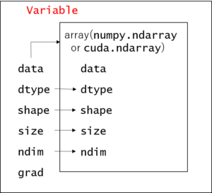
Variable
Variable class. It holds several properties, and several properties behaves same as numpy array.
Chainer variable can be created by Variable constructor, which creates chainer.Variable class object.
When I write Variable, it means chainer’s class for Variable. Please do not confuse with the usual noun of “variable”.
Note: the reason why chainer need to use own Variable, Function class for the calculation instead of just using numpy is because back propagation is necessary during deep learning training. Variable holds its “calculation history” information and Function has backward method which is differencial function in order to process back propagation. See below for more details
from chainer import Variable
# creating numpy array
# this is `numpy.ndarray` class
a = np.asarray([1., 2., 3.], dtype=np.float32)

# chainer variable is created from `numpy.ndarray` or `cuda.ndarray` (explained later)
x = Variable(a)

print('a: ', a, ', type: ', type(a))
print('x: ', x, ', type: ', type(x))
In the above code, numpy data type is explicitly set as dtype=np.float32. If we don’t set data type, np.float64 may be used as default type in 64-bit environment. However such a precision is usually “too much” and not necessary in machine learning. It is better to use lower precision for computational speed & memory usage.
attribute
Chainer Variable has following attributes
data
dtype
shape
ndim
size
grad
They are very similar to numpy.ndarray. You can access following attributes.
# These attributes return the same

print('attributes', 'numpy.ndarray a', 'chcainer.Variable x')
print('dtype', a.dtype, x.dtype)
print('shape', a.shape, x.shape)
print('ndim', a.ndim, x.ndim)
print('size', a.size, x.size)
attributes numpy.ndarray a chcainer.Variable x
dtype float32 float32
shape (3,) (3,)
ndim 1 1
size 3 3
# Variable class has debug_print function, to show this Variable's properties.
x.debug_print()
One exception is data attribute, chainer Variable‘s data refers numpy.ndarray
# x = Variable(a)

# `a` can be accessed via `data` attribute from chainer `Variable`
print('x.data is a : ', x.data is a)  # True -> means the reference of x.data and a are same.
print('x.data: ', x.data)
x.data is a :  True
x.data:  [ 1.  2.  3.]
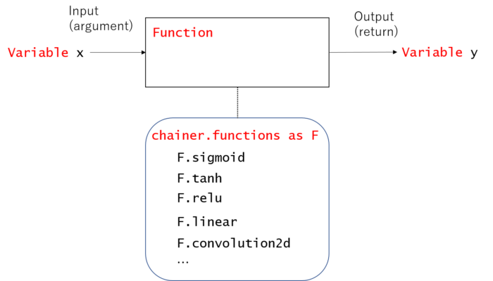
Function
1. Its input/output is Variable 2. chainer.functions provides many implementations of Function
We want to process some calculation to Variable. Variable can be calculated using
arithmetric operation (Ex. +, -, *, /)
method which is subclass of chainer.Function (Ex. F.sigmoid, F.relu)
# Arithmetric operation example
x = Variable(np.array([1, 2, 3], dtype=np.float32))
y = Variable(np.array([5, 6, 7], dtype=np.float32))

# usual arithmetric operator (this case `*`) can be used for calculation of `Variable`
z = x * y
print('z: ', z.data, ', type: ', type(z))
Only basic calculation can be done with arithmetric operations.
Chainer provides a set of widely used functions via chainer.functions, for example sigmoid function or ReLU (Rectified Linear Unit) function which is popularly used as activation function in deep learning.
# Functoin operation example
import chainer.functions as F

x = Variable(np.array([-1.5, -0.5, 0, 1, 2], dtype=np.float32))
sigmoid_x = F.sigmoid(x)  # sigmoid function. F.sigmoid is subclass of `Function`
relu_x = F.relu(x)        # ReLU function. F.relu is subclass of `Function`

print('x: ', x.data, ', type: ', type(x))
print('sigmoid_x: ', sigmoid_x.data, ', type: ', type(sigmoid_x))
print('relu_x: ', relu_x.data, ', type: ', type(relu_x))
Note: You can find capital letter of Function like F.Sigmoid or F.ReLU. Basically, these capital letter is actual class implmentation of Function while small letter method is getter method of these capital lettered instance.
It is recommended to use small letter method when you use F.xxx.
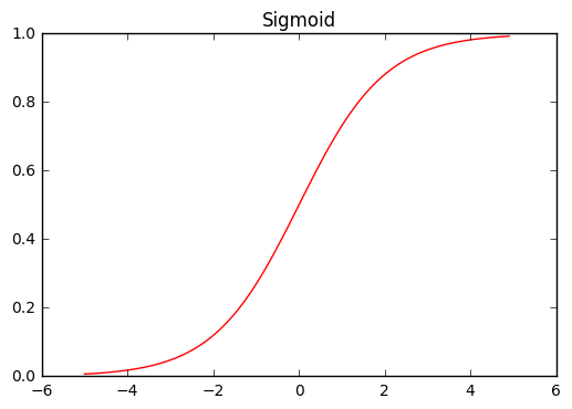
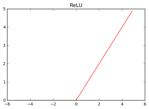
Just a side note, sigmoid and ReLU function are non-linear function whose form is like this.
%matplotlib inline
import matplotlib.pyplot as plt


def plot_chainer_function(f, xmin=-5, xmax=5, title=None):
    """draw graph of chainer `Function` `f`

    :param f: function to be plotted
    :type f: chainer.Function
    :param xmin: int or float, minimum value of x axis
    :param xmax: int or float, maximum value of x axis
    :return:
    """
    a = np.arange(xmin, xmax, step=0.1)
    x = Variable(a)
    y = f(x)
    plt.clf()
    plt.figure()
    # x and y are `Variable`, their value can be accessed via `data` attribute
    plt.plot(x.data, y.data, 'r')
    if title is not None:
        plt.title(title)
    plt.show()

plot_chainer_function(F.sigmoid, title='Sigmoid')
plot_chainer_function(F.relu, title='ReLU')
sigmoid function. It takes the value between 0 and 1. It saturates to 0 when x goes to negative infinity value, and saturates to 1 when x goes to positive infinity.relu (rectified linear unit) function. When x is negative it always returns 0, and when x is positive it behaves like identity map.
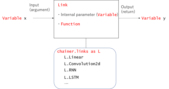
Link
1. Link acts like Function but it contains internal parameter to tune behavior 2. chainer.links provides many implementations of Link
Link is similar to Function, but it owns internal parameter. This internal parameter is tuned during training of machine learning.
Link is similar notion of Layer in caffe. Chainer provides layers which is introduced in popular papers via chainer.links. For example, Linear layer, Convolutional layer.
Let’s see the example, (below explanation is almost same with official tutorial)
L.Linear is one example of Link. 1. L.Linear holds Internal parameter self.W and self.b 2. L.Linear computes function, F.linear. Its output depends on internal parameter W and b.
import chainer.links as L

in_size = 3  # input vector's dimension
out_size = 2  # output vector's dimension

linear_layer = L.Linear(in_size, out_size)  # L.linear is subclass of `Link`

"""linear_layer has 2 internal parameters `W` and `b`, which are `Variable`"""
print('W: ', linear_layer.W.data, ', shape: ', linear_layer.W.shape)
print('b: ', linear_layer.b.data, ', shape: ', linear_layer.b.shape)
Note that internal parameter W is initialized with a random value. So every time you execute above code, the result will be different (try and check it!).
This Linear layer will take 3-dimensional vectors [x0, x1, x2…] (Variable class) as input and outputs 2-dimensional vectors [y0, y1, y2…] (Variable class).
In equation form,where i = 0, 1, 2... denotes each “minibatch” of input/output.
[Note] See source code of Linear class, you can easily understand it is just calling F.linear by
Let me emphasize the difference between Link and Function. Functions input-output relationship is fixed. On the other hand,Link` module has internal parameter and the function behavior can be changed by modifying (tuning) this internal parameter.
# Force update (set) internal parameters
linear_layer.W.data = np.array([[1, 2, 3], [0, 0, 0]], dtype=np.float32)
linear_layer.b.data = np.array([3, 5], dtype=np.float32)
# below is same code with above cell, but output data y will be different
x0 = np.array([1, 0, 0], dtype=np.float32)
x1 = np.array([1, 1, 1], dtype=np.float32)

x = Variable(np.array([x0, x1], dtype=np.float32))
y = linear_layer(x)
print('W: ', linear_layer.W.data)
print('b: ', linear_layer.b.data)
print('x: ', x.data)  # input is x0 & x1
print('y: ', y.data)  # output is y0 & y1
The value of output y is different compared to above code, even though we input same value of x.
These internal parameters are “tuned” during training in machine learning. Usually, we do not need to set these internal parameter W or b manually, chainer will automatically update these internal parameters during training through back propagation.
Chain
Chain is to construct neural networks. It usually consists of several combination of Link and Function modules.
Let’s see example,
from chainer import Chain, Variable


# Defining your own neural networks using `Chain` class
class MyChain(Chain):
    def __init__(self):
        super(MyChain, self).__init__()
        with self.init_scope():
            self.l1 = L.Linear(2, 2)
            self.l2 = L.Linear(2, 1)

    def __call__(self, x):
        h = self.l1(x)
        return self.l2(h)


x = Variable(np.array([[1, 2], [3, 4]], dtype=np.float32))

model = MyChain()
y = model(x)

print('x: ', x.data)  # input is x0 & x1
print('y: ', y.data)  # output is y0 & y1
Memo: Above init_scope() method is introduced in chainer v2, and Link class instances are initialized inside this scope.
In chainer v1, Chain was initialized as follows. Concretely, Link class instances are initialized in the argument of super method. For backward compatibility, you may use this type of initialization in chainer v2 as well.
from chainer import Chain, Variable


# Defining your own neural networks using `Chain` class
class MyChain(Chain):
    def __init__(self):
        super(MyChain, self).__init__(
            l1=L.Linear(2, 2),
            l2=L.Linear(2, 1)
        )

    def __call__(self, x):
        h = self.l1(x)
        return self.l2(h)


x = Variable(np.array([[1, 2], [3, 4]], dtype=np.float32))

model = MyChain()
y = model(x)

print('x: ', x.data)  # input is x0 & x1
print('y: ', y.data)  # output is y0 & y1
If you are using caffe, it is easy to get accustomed to chainer modules. Several variable’s functionality is similar and you can see below table for its correspondence.
I will summarize Chainer Advent Calendar 2016, to introduce what kind of deep learning projects are going on in Japan.
Chainer
Deep learning framework, chainer, is developed by Japanese company Preferred Networks and the community is quite active in Japan. Since interesting projects are presented and discussed, I would like to introduce them by summarizing it in English.
Advent Calendar
In Japan, there is a popular programming blog website called Qiita, and the “Advent Calendar” in Qiita is an event that interested people can join and write a blog for specific theme during Dec 1 to Dec 25.
If you want to read the details of each blog, you may use Google Translate Web to translate Japanese to English.
TL;DR
Based on personal interest, Day 25 and Day 14 were very interesting project (both of them are image processing related). Day 22 is must-read article for those who major image processing. Day 12 are quite interesting project in Reinforcement learning field.
For those who is interested in internal behavior of deep learning framework, Day 8 article is “rare” material that explains it in source code level in quite detail.
The project goal is given some image, it tries to say a joke about this image. By joining Convolutional Neural Network (CNN) to Recurrent Neural Network (RNN)
“Boke” is a Japanese word for saying joking, and there is a website “bokete“. Author collected teacher data from this website.
At first, it introduces how to use NStepLSTM in chainer. Then he implements Bi-directional LSTM in chainer and apply it to Chinese word segmentation task.
He introduces how back-end of deep learning framework works in chainer, by making 1 file size of “very light version of chainer”. I think it is quite good to understand how back propagation is implemented in deep learning framework.
Chord progression recognition task is music dictation task, the goal is to make a chord sequence of given music. It is categorized as sequence labeling problem, so this may applicable to another field too. He tried the task using the model DNN followed by CRF.
VIN (Value Iteration Networks) took the best award in NIPS 2016, which is a famous machine learning conference. This post summarizes/introduces VIN and implemented in Chainer and tested its performance.
In reinforcement learning, DQN is quite popular but it still needs to learn the model independently if the environment changes. VIN has more general adaptive power that it does not require so much environment knowledge to estimate the future value function.
The task is to detect the 5 edges of star ☆ in the picture. And he achieve the task using Convolution and Deconvolution Network. He made the data by himself.
Day 14. Change the style of picture into “Shinkai Makoto” style
Makoto Shinkai is a director of “Kiminonaha” (Your name), which is now big hit anime movie in Japan. He took his own picture and changed the style of that picture based on the style of “Kiminonaha”.
1. Explain how to train your own model in image classification task, starting from how to prepare image set data.
2. Creating a Web server in python to access model from browser. If you are thinking to make web service with some deep learning algorithm working in background, this is a good introduction tutorial.
Day 16. Try implementing abstraction layer of Chainer
He made a library to use chainer in scikit-learn way. Given data, the model can be parameterized (trained) using fit and predict, predict_proba can be used to use this trained model in scikit-learn.
With his library, now chainer can be used as follows,
category: chainer library, client browser usage of Chainer
For now, Chainer works only with python, there is no straight way to use Chainer in browser client environment. On the otherhand, another deep learning framework, keras, has Keras.js which enables keras model to work in browser environment using javascript.
He tried the following procedure
Train model with Chainer
Make the same model with Keras
Copy trained parameter from chainer to keras (he made library to copy parameter)
Convert Keras model into keras.js model
Run the model in browser client environment
There is after story,,, after this blog post, Keras developer Francois Chollet commented in Twitter in Japanese,
He further improved the model that user is allowed to put a color to indicate what color you want to use around this area. Now neural network put a color based on the request color given in the input image.
In Python, single-quoted strings and double-quoted strings are the same. This PEP does not make a recommendation for this. Pick a rule and stick to it. When a string contains single or double quote characters, however, use the other one to avoid backslashes in the string. It improves readability.
For triple-quoted strings, always use double quote characters to be consistent with the docstring convention in PEP 257 .
Explains behavior of print function in python 3 (or use from __future__ import print_function in python 2)
comma: , ー variable arguments
print function can take several arguments and they are printed with space (separate word specified by sep)
# default sep=' '
print('ab', 'cd', 'ef')             # ab cd ef
optional arguments
sep: specify separator word. default value is ' '
end: end of the text. default value is '\n'
file: output stream. default value is 'sys.stdout'
print('ab', 'cd', 'ef', sep=' ', end='\n', file=sys.stdout)  # default arg, same with above
print('ab', 'cd', 'ef', sep='SEP')  # abSEPcdSEPef
print('ab', 'cd', 'ef', end='\t')   # default end='\n'
print('gh', 'ij', 'kl', end='\t')
print(('ab', 'cd', 'ef'))           # ab cd ef	gh ij kl	('ab', 'cd', 'ef')

# write to file
f = open('test.txt', 'w')
print('hello world', file=f)
+ - string addition
print('hello' + 'world' + str(3)) # helloworld3
string can be concatenated with +. For number, you need to cast with str().
% and .format() ー formatting string
Refer PyFormat page for detailed explanation and its usage example.
Summary: use .format() since it is newer method than % and supports more functionality (for example center alignment, keyword arguments etc).
Ex.
# % or .format() usage
print('%d %d' % (3, 5))      # 3 5  old style
print('{} {}'.format(3, 5))  # 3 5  new style
Left-align, right-align, truncate
# left align, right align
print('%-10sm%10s' % ('left', 'right',))       # left      m     right
print('{:<10}m{:>10}'.format('left', 'right')) # left      m     right
# truncate
print('%.5s' % ('xylophone',))       # xylop
print('{:.5}'.format('xylophone',))  # xylop
These are the examples only .format() supports
# center align
print('{:^10}'.format('test'))  # '   test   '
# keyword argument
person = {'first': 'Jean-Luc', 'last': 'Picard'}
print('{p[first]} {p[last]} is {age} years old'.format(p=person, age=3))
Conclusion and summary
Use print() for python 3 compatibility. write from __future__ import print_function in python 2
Use , (multiple argument) when you want to print out several variables.


 where
where