
[Update 2017.06.11] Add chainer v2 code.
Contents
Training MNIST
You already studied basics of Chainer and MNIST dataset. Now we can proceed to the MNIST classification task. We want to create a classifier that classifies MNIST handwritten image into its digit. In other words, classifier will get array which represents MNIST image as input and outputs its label.
※ Chainer contains modules called Trainer, Iterator, Updater, which makes your training code more organized. It is quite nice to write your training code by using them in higher level syntax. However, its abstraction makes difficult to understand what is going on during the training. For those who want to learn deep learning in more detail, I think it is nice to know “primitive way” of writing training code. Therefore, I intentionally don’t to use these modules at first to explain training code.
The source code below is based on train_mnist_1_minimum.py.
[hands on] Before going to read the explanation, try to execute train_mnist_1_minimum.py. If you are using IDE like pycharm, just press run button. If you are going to run from command line, go to src directory first and execute
python mnist/train_mnist_1_minimum.py
You can see the log like below, indicating that the loss in decreasing through the training and accuracy is increasing.
GPU: -1# unit: 50# Minibatch-size: 100# epoch: 20out directory: result/1_minimumepoch 1train mean loss=0.41262895802656807, accuracy=0.8860333333909511, throughput=54883.71423542936 images/sectest mean loss=0.21496000131592155, accuracy=0.9357000035047531epoch 2train mean loss=0.1967763691022992, accuracy=0.942733335296313, throughput=66559.17396858479 images/sectest mean loss=0.17020921929739416, accuracy=0.9499000030755996epoch 3train mean loss=0.1490274258516729, accuracy=0.9558166695634523, throughput=66375.93210754421 images/sectest mean loss=0.1352944350033067, accuracy=0.9595000040531159...
Of course, it is ok that you may not understand the meaning of this log here. I will explain the detail one by one in the following.
Define Network and loss function
Let’s adopt Multi Layer Perceptron (MLP), which is a most simple neural network, as our model. This is written as follows with Chainer,
class MLP(chainer.Chain):
    """Neural Network definition, Multi Layer Perceptron"""
    def __init__(self, n_units, n_out):
        super(MLP, self).__init__()
        with self.init_scope():
            # the size of the inputs to each layer will be inferred when `None`
            self.l1 = L.Linear(None, n_units)  # n_in -> n_units
            self.l2 = L.Linear(None, n_units)  # n_units -> n_units
            self.l3 = L.Linear(None, n_out)    # n_units -> n_out

    def __call__(self, x):
        h1 = F.relu(self.l1(x))
        h2 = F.relu(self.l2(h1))
        y = self.l3(h2)
        return y
[Memo] In chainer v1, it was written as follows,
# Neural Network definition, Multi Layer Perceptron
class MLP(chainer.Chain):

    def __init__(self, n_units, n_out):
        super(MLP, self).__init__(
            # the size of the inputs to each layer will be inferred
            l1=L.Linear(None, n_units),  # n_in -> n_units
            l2=L.Linear(None, n_units),  # n_units -> n_units
            l3=L.Linear(None, n_out),  # n_units -> n_out
        )

    def __call__(self, x):
        h1 = F.relu(self.l1(x))
        h2 = F.relu(self.l2(h1))
        y = self.l3(h2)
        return y
This model is graphically drawn as follows. All nodes are fully connected, and the network with this kinds of structure is called MLP (Multi layer perceptron).
The fast part is input layer and the last part is output layer. The rest middle part of the layer is called “hidden layer”. This example contains only 1 hidden layer, but hidden layers may exist more than 1 in general (If you construct the network deeper, the number of hidden layer increases).
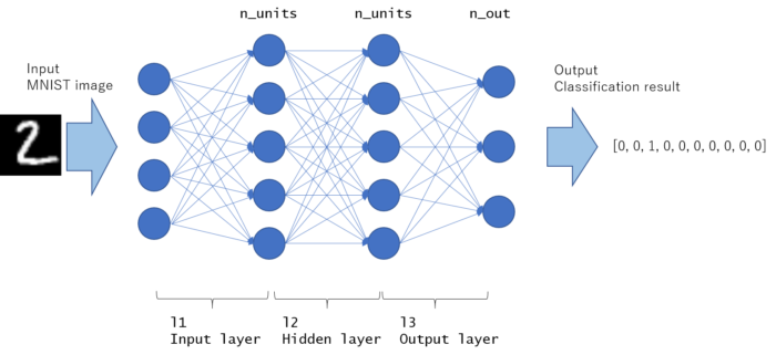
As written in __call__ function, it will take x (array indicating image) as input and return y (indicating predicted probability for each label) as output.
However, this is not enough for training the model. We need loss function to be optimized. In classification task, softmax cross entropy loss is often used.
Output of Linear layer can take arbitrary real number, Softmax function converts it into between 0-1, thus we can consider it as “probability for this label”. Cross entropy is to calculate loss between two probability distributions. Chainer has utility function F.softmax_cross_entropy(y, t) to calculate softmax of y followed by cross entropy with t. Loss will be smaller if the probability distribution predicted as y is equal to the actual probability distribution t. Intuitively, loss decreases when model can predict correct label given image.
Here I will skip more detail explanation, please study by yourself. Here is some reference,
To calculate softmax cross entropy loss, we define another Chain class, named SoftmaxClassifier as follows,
class SoftmaxClassifier(chainer.Chain):
    def __init__(self, predictor):
        super(SoftmaxClassifier, self).__init__(
            predictor=predictor
        )

    def __call__(self, x, t):
        y = self.predictor(x)
        self.loss = F.softmax_cross_entropy(y, t)
        self.accuracy = F.accuracy(y, t)
        return self.loss
Then, the model is instantiated as
    unit = 50  # Number of hidden layer units
    ...
    # Set up a neural network to train
    model = MLP(unit, 10)
    # Classifier will calculate classification loss, based on the output of model
    classifier_model = SoftmaxClassifier(model)
First, MLP model is created. n_out is set to 10 because MNIST has 10 patterns, from 0 until 9, in label. Then classifier_model is created based on the MLP model as its predictor. As you can see here, Network of Chain class can be “chained” to construct new network which is also Chain class. I guess this is the reason the name “Chainer” comes from.
Once loss function calculation is defined in __call__ function of model, you can set this model into Optimizer to proceed training.
    # Setup an optimizer
    optimizer = chainer.optimizers.Adam()
    optimizer.setup(classifier_model)
As already explained at Chainer basic module introduction 2, training proceeds by calling
            # Pass the loss function (Classifier defines it) and its arguments
            optimizer.update(classifier_model, x, t)
This code will calculate the loss as classifier_model(x, t) and tune (optimize) internal paramaters of model with Optimizer’s algorithm (Adam in this case).
Note that Back propagation is done automatically inside this update code, so you don’t need to write these codes explicitly.
As explain below, we will pass x and t in minibatch unit.
Use GPU
Chainer support GPU for calculation speed-up. To use GPU, PC must have NVIDIA GPU and you need to install CUDA, and better to install cudnn followed by installing chainer.
To write GPU compatible code, just add these 3 lines.
    if gpu >= 0:
        chainer.cuda.get_device(gpu).use()  # Make a specified GPU current
        classifier_model.to_gpu()           # Copy the model to the GPU
    xp = np if gpu < 0 else cuda.cupy
You need to set gpu device id in variable gpu.
If you don’t use gpu, set gpu=-1, which indicates not to use GPU and only use CPU. In that case numpy (written as np in above) is used for array calculation.
If you want to use gpu, set gpu=0 etc (usual consumer PC with NVIDIA GPU contains one GPU core, thus only gpu device id=0 can be used. GPU cluster have several GPUs (0, 1, 2, 3 etc) in one PC). In this case, call chainer.cuda.get_device(gpu).use() for specifying which GPU device to be used and model.to_gpu() to copy model’s internal parameters into GPU. In this case cupy is used for array calculation.
cupy
In python science calculation, numpy is widely used for vector, matrix and general tensor calculation. numpy will optimize these linear calculation with CPU automatically. cupy can be considered as GPU version of numpy, so that you can write GPU calculation code almost same with numpy. cupy is developed by Chainer team, as chainer.cuda.cupy in Chainer version 1.
However, cupy itself can be used as GPU version of numpy, thus applicable to more wide use case, not only for chainer. So cupy will be independent from chainer, and provided as cupy module from Chainer version 2.
GPU performance
How much different if GPU can be used? Below table show the image throughput with the model’s hidden layer unit size
| unit | CPU: Intel Core i7-6700 K Quad-core 4GHz | GPU: NVIDIA 980 Ti 2816 CUDA core 1 GHz base clock | How many times faster? |
| 1000 | 5500 | 38000 | ×6.9 |
| 3000 | 700 | 13000 | ×18.6 |
When the neural network size is large, many calculation can be parallelized and GPU advantage affect more. In some cases, GPU is about 20 times faster than CPU.
[Hands on] If you have NVIDIA GPU, compare the performance between CPU & GPU in your environment.
Train and Evaluation (Test)
train_mnist_1_minimum.py consists of 2 phase, training phase and evaluation (test) phase.
In regression/classification task in machine learning, you need to verify the model’s generalization performance. Even loss is decreasing with training dataset, it is not always true that loss for test (unseen) dataset is small.
Especially, we should take care overfitting problem. To cooperate this, you can check test dataset loss also decreases through the training.
Training phase
optimizer.updatecode will update model’s internal parameter to decrease loss.- Random permutation is to get random sample for constructing minibatch.
If training loss is not decreasing from the beginning, the root cause may be bug or some hyper parameter setting is wrong. When training loss stops decreasing (saturated), it is ok to stop the training.
        # training
        perm = np.random.permutation(N)
        sum_accuracy = 0
        sum_loss = 0
        start = time.time()
        for i in six.moves.range(0, N, batchsize):
            x = chainer.Variable(xp.asarray(train[perm[i:i + batchsize]][0]))
            t = chainer.Variable(xp.asarray(train[perm[i:i + batchsize]][1]))

            # Pass the loss function (Classifier defines it) and its arguments
            optimizer.update(classifier_model, x, t)

            sum_loss += float(classifier_model.loss.data) * len(t.data)
            sum_accuracy += float(classifier_model.accuracy.data) * len(t.data)
        end = time.time()
        elapsed_time = end - start
        throughput = N / elapsed_time
        print('train mean loss={}, accuracy={}, throughput={} images/sec'.format(
            sum_loss / N, sum_accuracy / N, throughput))
Evaluation (test) phase
- We must not call
optimizer.updatecode. Test dataset is considered as unseen data for model. Should not be included as training information. - We don’t need to take random permutation in test phase, only
sum_lossandsum_accuracyis necessary.
Evaluation code does (should have) no affect to model. This is just to check loss for test dataset. Ideal pattern is of course test loss decreases through the training.
        # evaluation
        sum_accuracy = 0
        sum_loss = 0
        for i in six.moves.range(0, N_test, batchsize):
            index = np.asarray(list(range(i, i + batchsize)))
            x = chainer.Variable(xp.asarray(test[index][0]))
            t = chainer.Variable(xp.asarray(test[index][1]))

            loss = classifier_model(x, t)
            sum_loss += float(loss.data) * len(t.data)
            sum_accuracy += float(classifier_model.accuracy.data) * len(t.data)

        print('test  mean loss={}, accuracy={}'.format(
            sum_loss / N_test, sum_accuracy / N_test))
| 1234567891011121314 | # evaluation sum_accuracy = 0 sum_loss = 0 for i in six.moves.range(0, N_test, batchsize): index = np.asarray(list(range(i, i + batchsize))) x = chainer.Variable(xp.asarray(test[index][0])) t = chainer.Variable(xp.asarray(test[index][1])) loss = classifier_model(x, t) sum_loss += float(loss.data) * len(t.data) sum_accuracy += float(classifier_model.accuracy.data) * len(t.data) print(‘test mean loss={}, accuracy={}’.format( sum_loss / N_test, sum_accuracy / N_test)) |
If this test loss is not decreasing while training loss is decreasing, it is a sign that model is overfitting. Then, you need to take action
- Increase the data size (if possible).
– Data augmentation is one method to increase the data effectively. - Decrease the number of internal parameters in neural network
– Try more simple network - Add Regularization term
Put all codes together,
"""
Very simple implementation for MNIST training code with Chainer using
Multi Layer Perceptron (MLP) model

This code is to explain the basic of training procedure.

"""
from __future__ import print_function
import time
import os
import numpy as np
import six

import chainer
import chainer.functions as F
import chainer.links as L
from chainer import cuda
from chainer import serializers


class MLP(chainer.Chain):
    """Neural Network definition, Multi Layer Perceptron"""
    def __init__(self, n_units, n_out):
        super(MLP, self).__init__(
            # the size of the inputs to each layer will be inferred
            l1=L.Linear(None, n_units),  # n_in -> n_units
            l2=L.Linear(None, n_units),  # n_units -> n_units
            l3=L.Linear(None, n_out),  # n_units -> n_out
        )

    def __call__(self, x):
        h1 = F.relu(self.l1(x))
        h2 = F.relu(self.l2(h1))
        y = self.l3(h2)
        return y


class SoftmaxClassifier(chainer.Chain):
    """Classifier is for calculating loss, from predictor's output.
    predictor is a model that predicts the probability of each label.
    """
    def __init__(self, predictor):
        super(SoftmaxClassifier, self).__init__(
            predictor=predictor
        )

    def __call__(self, x, t):
        y = self.predictor(x)
        self.loss = F.softmax_cross_entropy(y, t)
        self.accuracy = F.accuracy(y, t)
        return self.loss


def main():
    # Configuration setting
    gpu = -1                  # GPU ID to be used for calculation. -1 indicates to use only CPU.
    batchsize = 100           # Minibatch size for training
    epoch = 20                # Number of training epoch
    out = 'result/1_minimum'  # Directory to save the results
    unit = 50                 # Number of hidden layer units, try incresing this value and see if how accuracy changes.

    print('GPU: {}'.format(gpu))
    print('# unit: {}'.format(unit))
    print('# Minibatch-size: {}'.format(batchsize))
    print('# epoch: {}'.format(epoch))
    print('out directory: {}'.format(out))

    # Set up a neural network to train
    model = MLP(unit, 10)
    # Classifier will calculate classification loss, based on the output of model
    classifier_model = SoftmaxClassifier(model)

    if gpu >= 0:
        chainer.cuda.get_device(gpu).use()  # Make a specified GPU current
        classifier_model.to_gpu()           # Copy the model to the GPU
    xp = np if gpu < 0 else cuda.cupy

    # Setup an optimizer
    optimizer = chainer.optimizers.Adam()
    optimizer.setup(classifier_model)

    # Load the MNIST dataset
    train, test = chainer.datasets.get_mnist()

    n_epoch = epoch
    N = len(train)       # training data size
    N_test = len(test)  # test data size

    # Learning loop
    for epoch in range(1, n_epoch + 1):
        print('epoch', epoch)

        # training
        perm = np.random.permutation(N)
        sum_accuracy = 0
        sum_loss = 0
        start = time.time()
        for i in six.moves.range(0, N, batchsize):
            x = chainer.Variable(xp.asarray(train[perm[i:i + batchsize]][0]))
            t = chainer.Variable(xp.asarray(train[perm[i:i + batchsize]][1]))

            # Pass the loss function (Classifier defines it) and its arguments
            optimizer.update(classifier_model, x, t)

            sum_loss += float(classifier_model.loss.data) * len(t.data)
            sum_accuracy += float(classifier_model.accuracy.data) * len(t.data)
        end = time.time()
        elapsed_time = end - start
        throughput = N / elapsed_time
        print('train mean loss={}, accuracy={}, throughput={} images/sec'.format(
            sum_loss / N, sum_accuracy / N, throughput))

        # evaluation
        sum_accuracy = 0
        sum_loss = 0
        for i in six.moves.range(0, N_test, batchsize):
            index = np.asarray(list(range(i, i + batchsize)))
            x = chainer.Variable(xp.asarray(test[index][0]))
            t = chainer.Variable(xp.asarray(test[index][1]))

            loss = classifier_model(x, t)
            sum_loss += float(loss.data) * len(t.data)
            sum_accuracy += float(classifier_model.accuracy.data) * len(t.data)

        print('test  mean loss={}, accuracy={}'.format(
            sum_loss / N_test, sum_accuracy / N_test))

    # Save the model and the optimizer
    if not os.path.exists(out):
        os.makedirs(out)
    print('save the model')
    serializers.save_npz('{}/classifier_mlp.model'.format(out), classifier_model)
    serializers.save_npz('{}/mlp.model'.format(out), model)
    print('save the optimizer')
    serializers.save_npz('{}/mlp.state'.format(out), optimizer)

if __name__ == '__main__':
    main()