I joined Preferred Networks in December 2016 and leaving after eight years of work. I’d like to take a look back at what I was involved in.
For me, PFN can be described in one word as “a place that built up my confidence as an engineer”.
I majored in physics in university and had no experience in software development, such as competitive programming, and had no achievements in software development. However, looking back on the eight years at PFN, I feel that I had the opportunity to experience various things and grow a lot through working with talented people.
Worked on various collaborative research projects
I was first assigned to the new team as 2nd member (meaning there was only one “team member” before I joined), and we collaborated with various partner companies, mainly in the manufacturing industry, on cutting-edge issues.
It was a time when Deep Learning was emerging rapidly and gaining attention, and it was fun and challenging to work on the forefront issues from the top companies in all industries in Japan. It was also interesting for me to develop software that interacts with the real world rather than the closed in the web.
The projects were carried out with short periods of milestone setting, and as a result, the PDCA cycle turns very fast. Continuation of the project due to success or discontinuation of the project due to verification of technical uncertainty frequently occurs, and I feel that this also contributed to my growth.
Above all, my colleagues were extremely talented, and it was always stimulating to work with them, discussing and working together as a team to solve difficult problems.
OSS release and team launch
I was interested in applying Deep Learning to the field of science rather than popular field such as images or language. At that time, I participated in the IPAB Drug Discovery Contest, where we applied our domain knowledge and the then-popular Graph Neural Network (GNN) technology to achieve the Grand Prix, and we released the GNN implementation used for the contest as an OSS called Chainer Chemistry.
It was a great confidence booster for me to release an OSS, and I remember how much fun it was to implement various Neural Networks and verify their accuracy at that time. These activities led to the launch of several projects in the field of chemistry, and I was also involved in the launch of a new team.
Commercialization and JV launch 〜 Global expansion 〜
Around 2017, a joint research project to develop PFP, a foundational model for general-purpose atomistic simulation, was launched. Achieving commercialization from a seed research with cutting-edge technology to a product was something I had always wanted to achieve, and although there were various difficulties, the project finally resulted in the product release of Matlantis after two years of joint research.
Currently, it has been introduced to nearly 100 organizations, and global expansion has begun. As for the current generative AI, many technologies are at the forefront in the US, but I had always wanted to challenge the world with a SaaS product from Japan, especially in the field of science. Matlantis is a product that fulfills this desire, and I was fortunate enough to be involved in this project, which has a high degree of social contribution and I sympathize with the mission of PFCC, “Achieve a sustainable world by enabling the creation of innovative materials and materials.”
Development of a domestic LLM
Recently, I was involved in the post-training of the PLaMo-100B model.
It was a valuable experience to train a model of this size, which was almost unprecedented in Japan at the time. Even though I felt the pressure for this high target goal to make it usable, but it was also a unique experience to develop a model with the cooperation of many people.
(->A service based on this development, PLaMo Prime, has been released. Please check!)
Conclusion
I feel that I have been a generalist who connects various industries with the field of Deep Learning, rather than a specialist with specific industry expertise.
I was able to move to various fields, depending on my motivation, and I am grateful that I was able to experience various things.
The company’s phase has changed now, such as the commercialization of Plant, the release of Preferred AI, the release of Misemise, and the sales of PFCP and MN-Core, and I feel that the gears have completely shifted to the commercialization phase.
I will support the company from the outside as a fan, and I am looking forward to seeing its further progress in the daily news.
I am really grateful that I was able to work at this great workplace and appreciate those who worked with me, thank you very much!
* The document is a translation of original Japanese blog, translated by PLaMo (and modified a bit manually).
Since the emergence of generative AI like LLM, the pace of publishing papers in the industry has accelerated so fast. I’m trying so hard to keep up. I surveyed the methods/services to reach to the primary sources of trending AI research.
⭐⭐: I actively want to use.
⭐: I want to use.
🤖: The project which utilizes LLM.
Daily information source
Where to get source of the latest information everyday.
A page that summarizes and compiles updates from famous Twitter accounts, Discord servers of top companies in the AI field, and other social media platforms like Reddit. They use LLM (using Claude Opus as of April 2024) to summarize the content. Since they summarize global media, it seems particularly useful for grasping global corporate trends (especially for Japanese)!!
The initial sections, AI Reddit Recap, AI Twitter Recap, AI Discord Recap (or if it’s a bit older, just PART X: AI Twitter Recap and PART 0: Summary of Summaries of Summaries), seem like enough to read at first. They could be read in about 10 minutes.
You can see a summary of the Trending Papers that @AK updates daily.
It seems they carefully select highly relevant papers for each day, and since you can view them with thumbnails, it’s easy to see the authors and their affiliations. It looks like a good resource for those who want to check daily.
You can create lists by registering specific words and follow up the latest papers. It is useful to follow up about a week span. There used to be a “HOT” tag, but it seems to have disappeared now?
It’s a site mainly used for finding the implementation codes of papers or checking benchmark rankings. However, it seems like you can also find particularly noteworthy papers under the Trending Research section.
⭐X (Twitter)
Maybe it’s a good idea to follow specific individuals’ accounts. Just one star, as I don’t want to rely too much on Twitter.
Following specific authors might be a good idea. You can use the “Follow” button located at the top right of a person’s Google Scholar page to set up email notification when the author publishes new papers or updates.
You can check the citation graph of a paper, which allows you to visualize and display particularly influential papers based on citations and references to a specific paper.
Reference management tools
In a bonus chapter, let’s discuss how to manage the large volume of papers that come out every day.
The birth of ChatGPT is undoubtedly a technical breakthrough. Everyone surprised with its remarkably versatile responses across various domains. Some have even say, “The birth of ChatGPT marks the arrival of the singularity,” but in reality, the world hasn’t changed dramatically overnight.
Many of those following X may also feel that things haven’t changed dramatically, despite ChatGPT’s introduction.
First, let’s delve into ChatGPT and other Large Language Models (LLMs). From my understanding, Neural Networks (particularly the Transformer used in LLMs) exhibit a time complexity of at most O(N) to O(N^2) for a single inference, depending on the length N of the input text.
For example, solving NP-complete problems like the Traveling Salesman Problem (TSP) in polynomial time using Neural Networks seems unlikely (as solving it would imply P≠NP being solved as P=NP). Problems in the real world have inherent difficulties, much like having to physically traverse a certain distance (without teleportation) when traveling between two distant points. Solving problems of varying complexity requires a proportional amount of space (memory), time, and energy.
Diffusion Model is a trending model in the field of image generation. In this model, one needs to perform inference with the same model for a fixed number of diffusion steps (often in the thousands), regardless of the problem’s complexity.
Related to this, in the field of quantum computing, there exists something called the adiabatic theorem. This theorem states that the time required to transition accurately from an initial state A to the answer state B depends on the difficulty of the problem (in quantum adiabatic computation, problems are defined by the time evolution of a Hamiltonian H). Simple problems can be solved in polynomial time, whereas challenging problems necessitate exponential amounts of time.
In essence, solving difficult problems takes time proportional to their complexity. This is analogous to increasing the diffusion steps in the Diffusion Model (in this sense, many image generation problems fall under “easy” problems that can be solved in polynomial time).
Given these considerations, it’s unlikely that AGI will lead to an “exponential” leap (solving problems that can’t be solved in polynomial time at high speed), even if it emerges. However, constant-factor speedups are possible, and if it’s a 10x improvement, it would mean compressing 100 years of technological progress into 10 years, which would still be a significant acceleration.
Currently, chess AI has surpassed human professional players. However, it’s not completely incomprehensible, and most moves can be understood upon later analysis. I believe that AI will be used in various domains in a similar way, where its decision-making processes become more transparent and interpretable with time.
“LLM+Search is Hot Lately: Chess, Shogi, and Go have seen computers surpassing humans through extensive evaluation and search driven by learning. With the compass of LLM, we can now explore intellectual spaces rather than just games. It’s exciting to see what discoveries lie ahead.”
There have been rumors circulating about a project at OpenAI referred to as “Q*,” quietly progressing behind the scenes. As reading material, the following sources caught my attention:
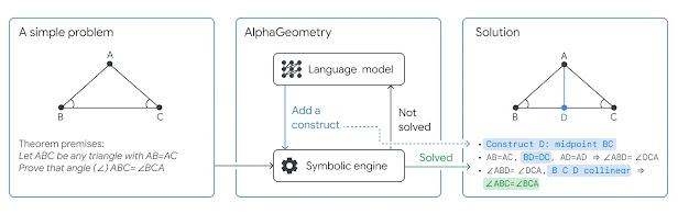
Recently, Google Deepmind published papers on “FunSearch” and “AlphaGeometry,” but there is potential for LLM+Search to be even more versatile and produce impactful results in this direction in the future.
So, what exactly does using LLM for search entail, and what are the recent trends in papers on this topic? Let’s explore that.
Breaking Down Tasks to Reach the Correct Answer
The first three papers I will introduce are more about breaking down thought processes rather than pure search. By properly breaking down the path to reaching a goal into steps and considering each one, we can improve the accuracy of arriving at the correct answer.
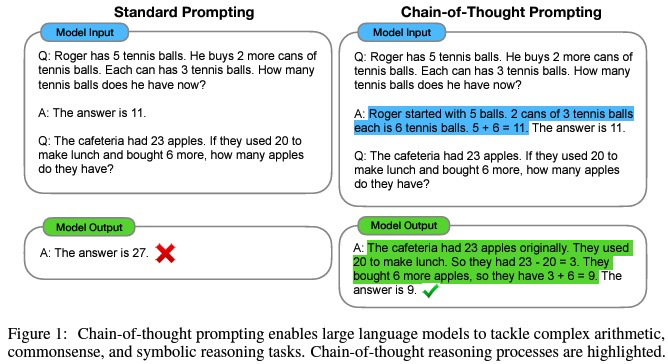
This paper demonstrates an improvement in answer accuracy by including the thought process leading to the answer when providing a few-shot example as a prompt. It is easier to understand by looking at concrete examples in the figure above. Rather than answering directly in one shot, including the intermediate steps in thinking and actually outputting the thought process allows us to reach the correct answer.
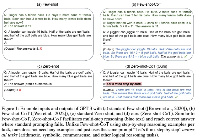
As a derivative, there is also something called Zero-shot-CoT.
In this case, the prompt is simpler, with just the phrase “Let’s think step by step.” This significantly improves answer accuracy and is very easy to use. This paper has been widely cited.
Similar to the original CoT, LLM can break down and think through the task according to the problem, even without including a few-shot example, simply by including the sentence “Let’s think step by step.” This approach leads to reaching the correct answer.
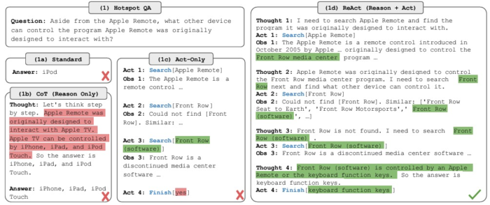
CoT focused solely on reasoning, while ReAct has improved its performance by incorporating “action“. For example web search action (more specifically, searching related text from Wikipedia and using it as input to complement LLM) is used in this paper.
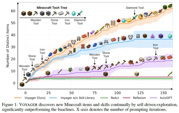
As an example of Open World Search using LLM, Voyager takes on the challenge of Minecraft.
It achieves better performance compared to the aforementioned ReAct and AutoGPT by incorporating unique innovations such as:
1. Automatic Curriculum
Determining the next sub tasks to solve. It considers new tasks that are not too difficult based on the current state. (LLM itself has some prior knowledge of Minecraft to some extent.)
2. Skill library
Functions of code, like equipping a sword and shield to defeat a zombie “combatZombie”, are encapsulated into skills and registered in a Skill Library. This allows them to be referenced and called upon later. By doing so, it is possible to reuse complex actions that have been successful in the past.
Skill Library references use embeddings based on the description text of this function, similar to RAG.
3. Iterative prompting mechanism
Considering the current environmental state and code execution errors to determine the next actions or modifications.
In this paper, the focus is on evaluating LLM’s ability for Open World Search. Instead of using image inputs or raw controller commands, it interacts with Minecraft through its API to obtain the current state and perform actions.
Utilizing LLM for exploration is demonstrated below,
By executing various code segments from LLM and observing their behavior, desired actions or skills are acquired.
Through the concept of the Skill Library, one can continually challenge more difficult tasks while incorporating their own growth.
While prior knowledge of Minecraft may have contributed to its success, the approach seems versatile and applicable to various tasks.
The following three papers are from DeepMind. In each case, LLM is used to search for outputs that increase the achievement score for tasks that can be quantitatively scored.
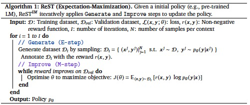
Rest^EM is a technique that combines ReST (Reinforced Self-Training) with EM (Expectation Maximization).
It comprises two steps:
1. Generate (E-step): The language model generates multiple output samples for each input context. Then, we filter these samples using a binary reward to collect the training dataset. 2. Improve (M-step): The original language model is supervised fine-tuned on the training dataset from the previous Generate step. The fine-tuned model is then used in the next Generate step.
E-step: In this step, LLM generates multiple candidate answers.
M-step: Among the generated candidates, the ones with good performance are selected as data to improve LLM.
This paper demonstrates that the proposed method works well for tasks that can be quantitatively evaluated.
MATH (Mathematical problem solving): Hendrycks’ MATH dataset
While the E-step uses the updated LLM, the M-step fine-tunes it from Pretrained weights each time. Overfitting appears to be a potential issue in this approach.
REST^EM is a simple self-training for LLM: 1) generate candidate solutions, 2) calculate rewards, 3) weigh each candidate with rewards and re-learn, repeat these. Effective in cases where automatic evaluation is possible, such as math and programming. https://t.co/5pK4tAnPVG
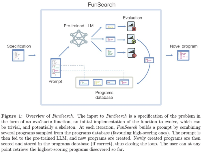
This paper from DeepMind, published in Nature, introduces FunSearch, short for Function space search. It employs LLM to search for better scores on challenging problems by seeking improved functions (solutions or algorithms). During the search, it uses an Evolutionary Algorithm to evolve and enhance algorithms while keeping the best-performing code alive.
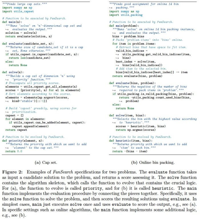
The paper successfully finds better algorithms than existing heuristic algorithms for two problems: the cap set problem and online bin packing (and some others in appendix).
The overall mechanism involves using a pretrained LLM (Codey, specialized for code generation) to generate candidate solutions, evaluating their scores, and saving the best ones in a “Programs database”.
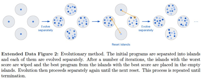
When generating the next set of candidates, an evolutionary algorithm is used to improve the solutions. This EA component seems to have a somewhat heuristic nature, and further improvements may be possible in the future.
Instead of asking it to create code from scratch, it provides task-specific templates and focuses on the core aspects of heuristic algorithms (e.g., priority, heuristic below) for the given problem. This kind of domain knowledge may be still necessary.
Another Nature paper from DeepMind, AlphaGeometry, shows that it was able to solve 25 out of 30 geometry problems in the International Mathematical Olympiad (IMO). It employs a Neuro Symbolic approach, transforming geometry problems into symbols for machine processing. The language model used here was trained on a dedicated dataset of 100 million samples, suggesting that it was developed specifically for this task rather than starting from a generic LLM.
Conclusion
The use of LLM allows for the automatic decomposition of complex problems into smaller tasks (path breakdown) during examination [CoT]. It also enables actions such as retrieving information from external sources and observing changes [ReAct, AutoGPT, Voyager]. Knowledge gained during the search process can be retained and effectively utilized in the future as “Skills” [Voyager], and the output can be improved iteratively [FunSearch]. Results from the search process can serve as learning data, specializing LLM for the specific task [Rest^EM].
However, it’s worth noting that Rest^EM, FunSearch, and AlphaGeometry all assume the ability to quickly evaluate the quality (reward) of the output solution. As a result, they seem to be limited to mathematical and coding problems at this stage.
Using LLM has made it easier to handle tasks with non-standard inputs and outputs, suggesting that there are still many applications to consider in the realm of exploration. Exciting developments in this area are anticipated in the future.
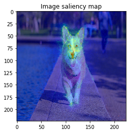
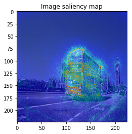
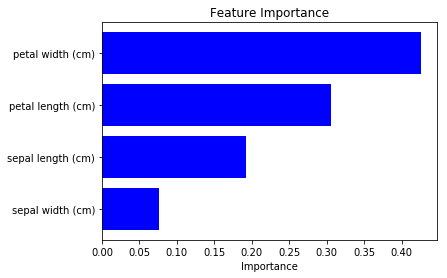
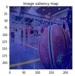
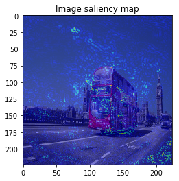
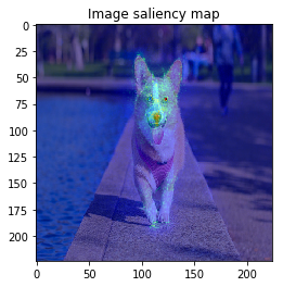
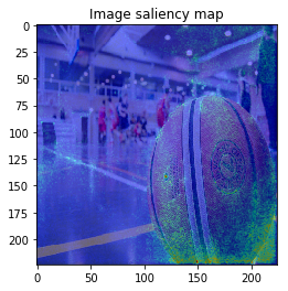
From left: 1. Classification saliency map visualization of VGG16, CNN model. 2. iris dataset feature importance calculation of MLP model. 3. Water solubility contribution visualization of Graph convolutional network model.
Abstract
Have you ever thought “Deep neural network is highly complicated black box, no one ever able to see what happens inside to result this output.”?
Even though NN consists of many layers and its mathematical analysis is difficult, there are some researches to show some saliency map like above images to understand model’s behavior or to get new knowledge for the dataset.
These saliency map calculation methods are implemented in Chainer Chemistry (even though the name contains “chemistry”, saliency module is available in many domains, as explained below). I will briefly explain how these work, and how to use it. You can also show these visualization figures after read this (a little bit long) article, enjoy!
It starts from theoretical explanation, followed by the code to use the module. Please jump to the “Examples” section if you just want to use it.
These methods calculate the contribution to the model’s prediction for each data.
※ Note that feature importance used in Random forest or XGBoost are calculated for the model. There is a difference that it is not calculated for “each data”.
Brief introduction – VanillaGrad
This method calculates derivative of output y with respect to input x, as a input contribution to the output prediction.
$$ s_i = \frac{dy}{dx_i} $$
Here, \(s_i\) is the saliency score, which is calculated for each input data’s \(i\)-th element \(x_i\). When the value of gradient is large for some element, the value change of this element results in big change of output prediction. So this element should have larger saliency (importance).
In terms of implementation, it is simply written as follows with chainer.
y = model(x)
y.backward()
s = x.grad
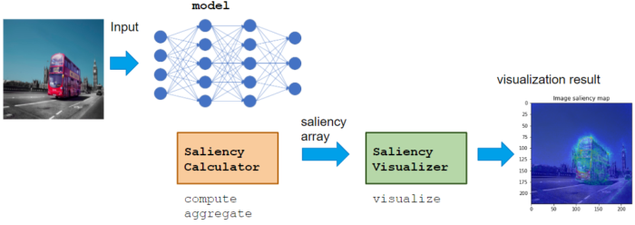
Saliency module usage
Calculator class calculates saliency score, like VaillaGrad, IntegratedGradient, or Occlusion.
Visualizer class visualizes calculated saliency score.
Calculator can be used with various NN model, which does not restrict the domain or application. Visualizer can be implemented to adopt Application for the proper visualization for the domain.
Basic usage flow is to call Calculator compute, aggregate -> Visualizer visualize
# model is chainer.Chain, x is dataset
calculator = GradientCalculator(model)
saliency_samples = calculator.compute(x)
saliency = calculator.aggregate(saliency_samples)

visualizer = ImageVisualizer()
visualizer.visualize(saliency)
Calculator class
Here I use GradientCalculator as an example which calcultes VanillaGrad explained above. Let’s see how to call each method.
Instantiation
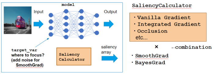
Instance with passing model, which is the target neural network to calculate saliency.
calculator = GradientCalculator(model)
compute method
compute method calculates “saliency samples” for each data x.
When calculating VanillaGrad, it suffices with M=1 since the calculation result of grad is always same. However, sampling is necessary when we consider SmoothGrad or BayesGrad.
I will explain SmoothGrad & BayesGrad to understand the notion of sampling.
– SmoothGrad –
Practically, VanillaGrad tends to show Noisy saliency map, so SmoothGrad suggests to change input x to shift a small ϵ, resulting input x+ϵ and calculate grad. We can take the average as the final saliency score.
$$s_{mi} = \frac{dy}{dx_i} |_{x=x+\epsilon_m}$$
$$s_{i} = \frac{1}{M} \sum_{m=1}^{M}{s_{mi}}$$
In the library, compute method calculates saliency sample \(s_{mi}\), and aggregate method calculates saliency
SmoothGrad changed input x by adding Gaussian noise, to take sampling. BayesGrad considers sampling along Neural Network parameter \(\theta\), trained with dataset D, to get prediction posterior distribution \(y_\theta \sim p(\theta|D)\) to take the sampling as follows:
Aggregation methods differ by paper by paper, aggregate method in the library supports following 3 method.
‘raw’: simply take average
$$ s_i = \frac{1}{M} \sum_{m}^{M} s_{mi} $$
‘abs’: take absolute average
$$ s_i = \frac{1}{M} \sum_{m}^{M} |s_{mi}| $$
‘square’: take squared average
$$ s_i = \frac{1}{M} \sum_{m}^{M} s_{mi}^2 $$
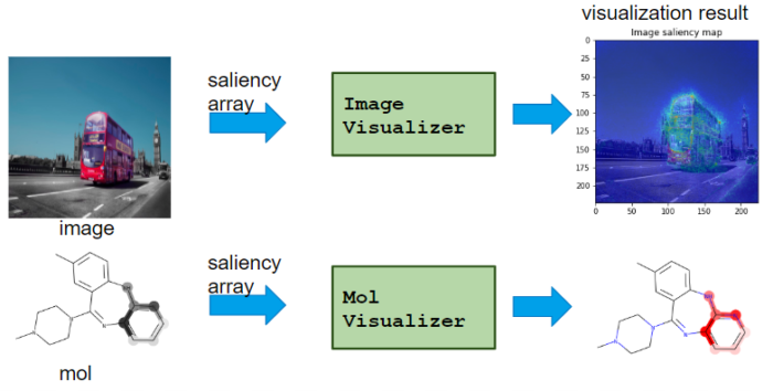
Visualizer class
It visualizes saliency from Calcualtor class.
– TableVisualizer: plot feature importance for each table data – ImageVisualizer: plot saliency map of image – MolVisualizer: plot saliency map of molecule
As shown, Visualizer differs for each application.
visualize method
Visualizer plots figure with visualize method.
Note that Calculator class calcultes saliency with batch, but visualizer visualizes one data, so you need to specify it.
# Instantiation
visualizer = ImageVisualizer()

# Visualize `i`-th data
i = 0
visualizer.visualize(saliency[i])
The figure can be saved by setting save_filepath argument.
# Save saliency map
visualizer.visualize(saliency[i], save_filepath='saliency.png')
Examples
It was a long explanation,,, now let’s use it!
Table data application: calculate feature importance
Neural Network is MLP (Multi Layer Parceptron), Dataset is iris dataset provided by sklearn.
iris dataset is to classify 3 flower species ‘setosa’, ‘versicolor’, ‘virginica’, from 4 features ‘sepal length (cm)’, ‘sepal width (cm)’, ‘petal length (cm)’, ‘petal width (cm)’.
# model
from chainer.functions import relu, dropout
from chainer_chemistry.models.mlp import MLP
from chainer_chemistry.models.prediction.classifier import Classifier

def activation_relu_dropout(h):
return dropout(relu(h), ratio=0.5)

out_dim = len(iris.target_names)
predictor = MLP(out_dim=out_dim, hidden_dim=48, n_layers=2, activation=activation_relu_dropout)
classifier = Classifier(predictor)

# dataset
import sklearn
from sklearn import datasets
import numpy as np
from chainer_chemistry.datasets.numpy_tuple_dataset import NumpyTupleDataset

iris = datasets.load_iris()
# All dataset is to train for simplicity
dataset = NumpyTupleDataset(iris.data.astype(np.float32), iris.target.astype(np.int32))
train = dataset
Model’s training code is omitted (please refer the code on github). After training the model, we can use saliency module.
First, use Calculator compute -> aggregate to calculate saliency.
Second, use Visualizer visualize method to plot figure.
from chainer_chemistry.saliency.visualizer.table_visualizer import TableVisualizer
from chainer_chemistry.saliency.visualizer.common import normalize_scaler

visualizer = TableVisualizer()
# Visualize saliency of `i`-th data
i = 0
visualizer.visualize(saliency_vanilla[i], feature_names=iris.feature_names,
scaler=normalize_scaler)
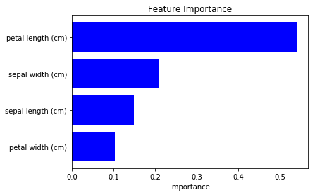
We can see how the each feature contributes to the final output prediction loss.
We saw saliency for 0-th data above, now we can calculate average along dataset to show feature importance for all data (which roughly corresponds to model’s feature importance).
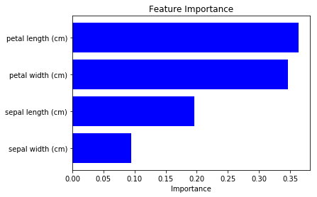
We can see “petal length” and “petal width” are more important. (note that the result differs according to the model’s training condition, be careful.)
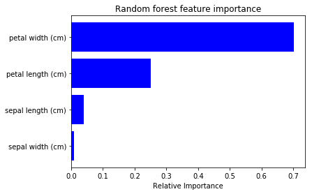
To check above result is plausible, I tried to plot feature impotance of Random Forest from sklearn (code).
Even though the absolute importance value differs, its order is same. So I feel the saliency calculation of NN is also useful for feature selection etc 🙂
Image data: show saliency map for classification task
Training CNN takes time, so I will use pre-trained model. I will use VGG16 model provided by Chainer this time.
from chainer.links.model.vision.vgg import VGG16Layers

predictor = VGG16Layers()
It automatically download pretrained parameters, with only this code.
ImageNet correct label name is downloaded from here.
import numpy as np

with open('imagenet1000_clsid_to_human.txt') as f:
lines = f.readlines()

def extract_value(s):
quote_str = s[s.index(':') + 2]
return s[s.find(quote_str)+1:s.rfind(quote_str)]

classes = np.array([extract_value(line) for line in lines])
from PIL import Image
import numpy as np

import chainer
import chainer.functions as F

# basketball, bus, dog
image_paths = ['./input/pexels-photo-945471.jpeg', './input/pexels-photo-45923.jpeg',
'./input/pexels-photo-58997.jpeg']

imgs = [Image.open(fp) for fp in image_paths]
x = xp.asarray([chainer.links.model.vision.vgg.prepare(img) for img in imgs])
with chainer.using_config('train', False):
result = predictor.forward(x, layers=['prob'])
prob = result['prob']

lables_pred = np.argsort(cuda.to_cpu(prob.array), axis=1)[:, ::-1]

for i in range(len(lables_pred)):
print('i', i, 'labels_pred', lables_pred[i, :5], classes[lables_pred[i, :5]])
`
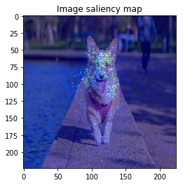
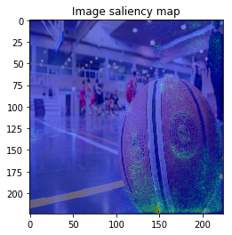
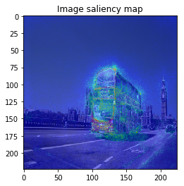
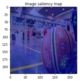
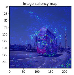
When we see the result, 1-st image is correctly predicted as Basketball, 2nd image is predicted as trailer truck though it is actually bus, 3rd image is predicted as basenji (ImageNet contains various dog’s species as label, I do not know this is indeed correct or not…).
VanillaGrad
So let’s proceed to saliency calculation. This time, I will calculate saliency for “why predicting the label of top prediction”, not for the ground truth label. For example in 2nd image, we calculate saliency for why the CNN model predicted “trailer truck”, so the ground truth label (and the model predicts correct label or not) is not related.
I can set output_var as “softmax cross entropy between top prediction label” (instead of ground truth label).
import chainer.functions as F
from chainer import cuda

def eval_fun(x):
result = predictor(x, layers=['fc8'])
out = result['fc8']
xp = cuda.get_array_module(out.array)
labels_pred = xp.argmax(out.array, axis=1).astype(xp.int32)
loss = F.softmax_cross_entropy(out, labels_pred)
return loss
Once eval_fun is defined, we can follow usual step: Calculator compute -> aggregate, ImageVisualizer visualize, to see the result.
We set ch_axis=2 in aggregate method, this is different from usual (minibatch, ch, h, w) image shape, because sampling_axis is added in front.
ImageVisualizer visualization result is as follows:
from chainer_saliency.visualizer.image_visualizer import ImageVisualizer

visualizer = ImageVisualizer()

for index in range(len(saliency_vanilla)):
image = imgs[index].resize(saliency_vanilla[index].shape)
visualizer.visualize(saliency_vanilla[index], image, show_colorbar=False)
It looks the model focuses on right place,,, but it is too noisy to see the result.
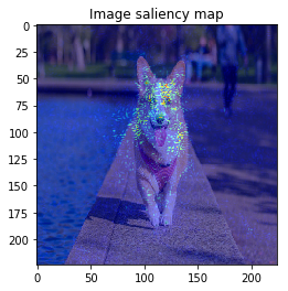
SmoothGrad
Next, let’s calculate SmoothGrad. We can set noise_sampler argument in Calculator compute method.
from chainer_chemistry.saliency.calculator.common import GaussianNoiseSampler

M = 30

# --- SmoothGrad ---
# 2. compute
saliency_samples_smooth = gradient_calculator.compute(x, M=M, noise_sampler=GaussianNoiseSampler())

# 3. aggregate
saliency_smooth = gradient_calculator.aggregate(
saliency_samples_smooth, ch_axis=2, method='abs')

for index in range(len(saliency_vanilla)):
image = imgs[index].resize(saliency_smooth[index].shape)
visualizer.visualize(saliency_smooth[index], image, show_colorbar=False)
aggregate, visualize methods are same with VanillaGrad.
The figure looks much better, we can see model focuses on the edge of objects.
BayesGrad
At last, we will try BayesGrad. It requires that the model has stochastic operation. This time, VGG16 has dropout operation so it is applicable.
To calculate BayesGrad, we only need to set train=True in Calculator compute method. Chainer automatically enables dropout so that output is different in each samples, results that we can calculate saliency samples (gradient) for prediction distribution.
When I try combining both SmoothGrad & BayesGrad, the result are as follows:
Molecule data: plot property contribution map for regression task
For regression task, we can calculate saliency to consider its sign, to show that the input contributes to positive or negative to the prediction.
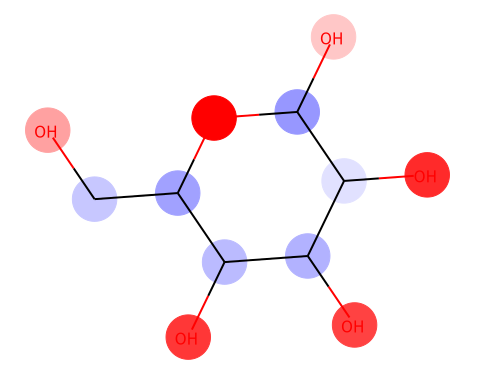
In this last example, I will use Graph convolution model in Chainer Chemistry, to visualize water solubility contribution for each atom.
ESOL dataset is used for water solubility dataset.
import numpy as np
import chainer
from chainer.functions import relu, dropout

from chainer_chemistry.models.ggnn import GGNN
from chainer_chemistry.datasets.numpy_tuple_dataset import NumpyTupleDataset
from chainer_chemistry.datasets.zinc import get_zinc250k
from chainer_chemistry.dataset.preprocessors.ggnn_preprocessor import GGNNPreprocessor
from chainer_chemistry.models.mlp import MLP
from chainer_chemistry.models.prediction.regressor import Regressor


# Model
def activation_relu_dropout(h):
    return dropout(relu(h), ratio=0.25)

class GraphConvPredictor(chainer.Chain):
    def __init__(self, graph_conv, mlp=None):
        """Initializes the graph convolution predictor.
        Args:
            graph_conv: The graph convolution network required to obtain
                        molecule feature representation.
            mlp: Multi layer perceptron; used as the final fully connected
                 layer. Set it to `None` if no operation is necessary
                 after the `graph_conv` calculation.
        """
        super(GraphConvPredictor, self).__init__()
        with self.init_scope():
            self.graph_conv = graph_conv
            if isinstance(mlp, chainer.Link):
                self.mlp = mlp
        if not isinstance(mlp, chainer.Link):
            self.mlp = mlp

    def __call__(self, atoms, adjs):
        x = self.graph_conv(atoms, adjs)
        if self.mlp:
            x = self.mlp(x)
        return x

n_unit = 32
conv_layers = 4
class_num = 1
device = 0  # -1 for CPU

ggnn = GGNN(out_dim=n_unit, hidden_dim=n_unit, n_layers=conv_layers)
mlp = MLP(out_dim=class_num, hidden_dim=n_unit, activation=activation_relu_dropout)
predictor = GraphConvPredictor(ggnn, mlp)
regressor = Regressor(predictor, device=device)

# Dataset
preprocessor = GGNNPreprocessor()

result = get_molnet_dataset('delaney', preprocessor, labels=None, return_smiles=True)
train = result['dataset'][0]
smiles = result['smiles'][0]
After training the model (see repository for the code), we can proceed to visualization.
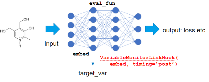
This time, we want to focus on contribution to the output prediction instead of loss. So we can define eval_fun to set output_var as predictor‘s output.
Also, we need to take care that input x is label of the node, gradient is not propagated until this input, we need to adopt gradient of the variable after embed layer, which is hidden layer’s variable.
In this kind of case, to set target_var as intermediate variable in the model, we can use VariableMonitorLinkHook.
I use IntegratedGradientsCalculator this time, to calculate saliency:
import chainer.functions as F

from chainer_chemistry.saliency.calculator.gradient_calculator import GradientCalculator
from chainer_chemistry.saliency.calculator.integrated_gradients_calculator import IntegratedGradientsCalculator
from chainer_chemistry.link_hooks.variable_monitor_link_hook import VariableMonitorLinkHook


def eval_fun(x, adj, t):
    pred = predictor(x, adj)
    pred_summed = F.sum(pred)
    return pred_summed

# 1. instantiation
calculator = IntegratedGradientsCalculator(
predictor, steps=5, eval_fun=eval_fun, target_extractor=VariableMonitorLinkHook(ggnn.embed, timing='post'),
device=device)
Red color shows the positive effect on solubility (Hydrophilic), blue color shows the negative effect on solubility (Hydrophobic).
Above figure matches the common sense of Hydrophilic effects usually occurs at polarization exists (OH), and we can see Hydrophobic effects where C-chain continues.
Conclusion
I introduced saliency module, which is highly flexible and applicable to any domain.
You can try all the examples with few machine resources, only with CPU, so please try!! (Saliency map visualization of image uses pre-trained model so only inference is necessary).
This post is based on the jupyter notebook ptb_dataset_introduction.ipynb uploaded on github.
Penn Treebank dataset, known as PTB dataset, is widely used in machine learning of NLP (Natural Language Processing) research.
Dataset if provided by the official page: Treebank-3
In Chainer, PTB dataset can be obtained with build-in function.
Let’s see the dataset structure.
from __future__ import print_function
import os
import matplotlib.pyplot as plt
%matplotlib inline

import numpy as np

import chainer
Download PTB dataset
chainer.datasets.get_ptb_words method is prepared in Chainer to get PTB dataset. Dataset is automatically downloaded from https://github.com/tomsercu/lstm/tree/master/data only for the first time, and its cache is used from second time.
train, val, test = chainer.datasets.get_ptb_words()
The dataset structure is numpy.ndarray.
train[i] represents i-th word in integer, which represents word ID.
ptb_word_id_dict = ptb_dict
ptb_id_word_dict = dict((v,k) for k,v in ptb_word_id_dict.items())

# Same with https://raw.githubusercontent.com/tomsercu/lstm/master/data/ptb.train.txt
print([ptb_id_word_dict[i] for i in train[:30]])
Now you can see that the sequence of word id is indeed a list of word which forms a meaningful text.
But list representation is little bit difficult to read for human, let’s convert to natural text using ' '.join() method.
# ' '.join() will convert list representation more readable

' '.join([ptb_id_word_dict[i] for i in train[:300]])
"aer banknote berlitz calloway centrust cluett fromstein gitano guterman hydro-quebec ipo kia memotec mlx nahb punts rake regatta rubens sim snack-food ssangyong swapo wachter <eos> pierre <unk> N years old will join the board as a nonexecutive director nov. N <eos> mr. <unk> is chairman of <unk> n.v. the dutch publishing group <eos> rudolph <unk> N years old and former chairman of consolidated gold fields plc was named a nonexecutive director of this british industrial conglomerate <eos> a form of asbestos once used to make kent cigarette filters has caused a high percentage of cancer deaths among a group of workers exposed to it more than N years ago researchers reported <eos> the asbestos fiber <unk> is unusually <unk> once it enters the <unk> with even brief exposures to it causing symptoms that show up decades later researchers said <eos> <unk> inc. the unit of new york-based <unk> corp. that makes kent cigarettes stopped using <unk> in its <unk> cigarette filters in N <eos> although preliminary findings were reported more than a year ago the latest results appear in today 's new england journal of medicine a forum likely to bring new attention to the problem <eos> a <unk> <unk> said this is an old story <eos> we 're talking about years ago before anyone heard of asbestos having any questionable properties <eos> there is no asbestos in our products now <eos> neither <unk> nor the researchers who studied the workers were aware of any research on smokers of the kent cigarettes <eos> we have no useful information on whether users are at risk said james a. <unk> of boston 's <unk> cancer institute <eos> dr. <unk> led a team of researchers from the national cancer institute and the medical schools of harvard university and boston university <eos> the <unk>"
print(' '.join([ptb_id_word_dict[i] for i in val[:300]]))
consumers may want to move their telephones a little closer to the tv set <eos> <unk> <unk> watching abc 's monday night football can now vote during <unk> for the greatest play in N years from among four or five <unk> <unk> <eos> two weeks ago viewers of several nbc <unk> consumer segments started calling a N number for advice on various <unk> issues <eos> and the new syndicated reality show hard copy records viewers ' opinions for possible airing on the next day 's show <eos> interactive telephone technology has taken a new leap in <unk> and television programmers are racing to exploit the possibilities <eos> eventually viewers may grow <unk> with the technology and <unk> the cost <eos> but right now programmers are figuring that viewers who are busy dialing up a range of services may put down their <unk> control <unk> and stay <unk> <eos> we 've been spending a lot of time in los angeles talking to tv production people says mike parks president of call interactive which supplied technology for both abc sports and nbc 's consumer minutes <eos> with the competitiveness of the television market these days everyone is looking for a way to get viewers more excited <eos> one of the leaders behind the expanded use of N numbers is call interactive a joint venture of giants american express co. and american telephone & telegraph co <eos> formed in august the venture <unk> at&t 's newly expanded N service with N <unk> computers in american express 's omaha neb. service center <eos> other long-distance carriers have also begun marketing enhanced N service and special consultants are <unk> up to exploit the new tool <eos> blair entertainment a new york firm that advises tv stations and sells ads for them has just formed a
print(' '.join([ptb_id_word_dict[i] for i in test[:300]]))
no it was n't black monday <eos> but while the new york stock exchange did n't fall apart friday as the dow jones industrial average plunged N points most of it in the final hour it barely managed to stay this side of chaos <eos> some circuit breakers installed after the october N crash failed their first test traders say unable to cool the selling panic in both stocks and futures <eos> the N stock specialist firms on the big board floor the buyers and sellers of last resort who were criticized after the N crash once again could n't handle the selling pressure <eos> big investment banks refused to step up to the plate to support the beleaguered floor traders by buying big blocks of stock traders say <eos> heavy selling of standard & poor 's 500-stock index futures in chicago <unk> beat stocks downward <eos> seven big board stocks ual amr bankamerica walt disney capital cities\/abc philip morris and pacific telesis group stopped trading and never resumed <eos> the <unk> has already begun <eos> the equity market was <unk> <eos> once again the specialists were not able to handle the imbalances on the floor of the new york stock exchange said christopher <unk> senior vice president at <unk> securities corp <eos> <unk> james <unk> chairman of specialists henderson brothers inc. it is easy to say the specialist is n't doing his job <eos> when the dollar is in a <unk> even central banks ca n't stop it <eos> speculators are calling for a degree of liquidity that is not there in the market <eos> many money managers and some traders had already left their offices early friday afternoon on a warm autumn day because the stock market was so quiet <eos> then in a <unk> plunge the dow
So how to implement custom extensions for trainer in Chainer? There are mainly 3 approaches.
Define function
Use decorator, @chainer.training.extension.make_extension
Define class
Most of the case, 1. Define function is the easiest way to quickly implement your extension.
1. Define function
Just a function can be a trainer extension. Simply, define a function which takes one argument (in below case “t”), which is trainer instance.
1-1. define function
    # 1-1. Define function for trainer extension
    def my_extension(t):
        print('my_extension function is called at epoch {}!'
              .format(t.updater.epoch_detail))
        # Change optimizer's learning rate
        optimizer.lr *= 0.99
        print('Updated optimizer.lr to {}'.format(optimizer.lr))

    trainer.extend(my_extension, trigger=(1, 'epoch'))
Here the argument of my_extension function, t, is trainer instance. You may obtain a lot of information related to the training procedure from trainer. In this case, I took the current epoch information by accessing updater’s property (trainer holds updater’s instance), t.updater.epoch_detail.
The extension is invoked based on the trigger configuration. In above code trigger=(1, 'epoch') means that this extension is invoked every once in one epoch.
Try changing the code from trainer.extend(my_extension, trigger=(1, 'epoch')) to trainer.extend(my_extension, trigger=(1, 'iteration')). Then the code is invoked every one iteration (Causion: it outpus the log very frequently, please stop it after executed and you have checked the behavior).
1-2. Use lambda
Instead of defining a function explicitly, you can simply use lambda function if the extension’s logic is simple.
    # Use lambda function for extension
    trainer.extend(lambda t: print('lambda function called at epoch {}!'
                                   .format(t.updater.epoch_detail)),
                   trigger=(1, 'epoch'))
"""Inference/predict code for simple_sequence dataset

model must be trained before inference,
train_simple_sequence.py must be executed beforehand.
"""
from __future__ import print_function

import argparse
import os
import sys

import matplotlib
import numpy as np

matplotlib.use('Agg')
import matplotlib.pyplot as plt
import chainer
import chainer.functions as F
import chainer.links as L
from chainer import training, iterators, serializers, optimizers, Variable, cuda
from chainer.training import extensions

sys.path.append(os.pardir)
from RNN import RNN
from RNN2 import RNN2
from RNN3 import RNN3
from RNNForLM import RNNForLM


def main():
    archs = {
        'rnn': RNN,
        'rnn2': RNN2,
        'rnn3': RNN3,
        'lstm': RNNForLM
    }

    parser = argparse.ArgumentParser(description='simple_sequence RNN predict code')
    parser.add_argument('--arch', '-a', choices=archs.keys(),
                        default='rnn', help='Net architecture')
    #parser.add_argument('--batchsize', '-b', type=int, default=64,
    #                    help='Number of images in each mini-batch')
    parser.add_argument('--unit', '-u', type=int, default=100,
                        help='Number of LSTM units in each layer')
    parser.add_argument('--gpu', '-g', type=int, default=-1,
                        help='GPU ID (negative value indicates CPU)')
    parser.add_argument('--primeindex', '-p', type=int, default=1,
                        help='base index data, used for sequence generation')
    parser.add_argument('--length', '-l', type=int, default=100,
                        help='length of the generated sequence')
    parser.add_argument('--modelpath', '-m', default='',
                        help='Model path to be loaded')
    args = parser.parse_args()

    print('GPU: {}'.format(args.gpu))
    #print('# Minibatch-size: {}'.format(args.batchsize))
    print('')

    train, val, test = chainer.datasets.get_ptb_words()
    n_vocab = max(train) + 1  # train is just an array of integers
    print('#vocab =', n_vocab)
    print('')

    # load vocabulary
    ptb_word_id_dict = chainer.datasets.get_ptb_words_vocabulary()
    ptb_id_word_dict = dict((v, k) for k, v in ptb_word_id_dict.items())

    # Model Setup
    model = archs[args.arch](n_vocab=n_vocab, n_units=args.unit)
    classifier_model = L.Classifier(model)
    if args.gpu >= 0:
        chainer.cuda.get_device(args.gpu).use()  # Make a specified GPU current
        classifier_model.to_gpu()  # Copy the model to the GPU
    xp = np if args.gpu < 0 else cuda.cupy

    if args.modelpath:
        serializers.load_npz(args.modelpath, model)
    else:
        serializers.load_npz('result/{}_ptb.model'.format(args.arch), model)

    # Dataset preparation
    prev_index = args.primeindex

    # Predict
    predicted_sequence = [prev_index]
    for i in range(args.length):
        prev = chainer.Variable(xp.array([prev_index], dtype=xp.int32))
        current = model(prev)
        current_index = np.argmax(cuda.to_cpu(current.data))
        predicted_sequence.append(current_index)
        prev_index = current_index

    predicted_text_list = [ptb_id_word_dict[i] for i in predicted_sequence]
    print('Predicted sequence: ', predicted_sequence)
    print('Predicted text: ', ' '.join(predicted_text_list))

if __name__ == '__main__':
    main()
Given the first text by the index, args.primeindex, model will predict the following sequence as word id.
The last three line converts the word id sequence into readable word sentence using ptb_id_word_dict.
    predicted_text_list = [ptb_id_word_dict[i] for i in predicted_sequence]
    print('Predicted sequence: ', predicted_sequence)
    print('Predicted text: ', ' '.join(predicted_text_list))
Result
When I run, (the model is RNN model)
$ python predict_ptb.py -p 553
I got the text
Predicted text: executive vice president and chief operating officer of <unk> <unk> & <unk> a <unk> mass. newsletter <eos> the <unk> <unk> <unk> <unk> <unk> <unk> from the <unk> <eos> the <unk> <unk> <unk> <unk> <unk> <unk> from the <unk> <eos> the <unk> <unk> <unk> <unk> <unk> <unk> from the <unk> <eos> the <unk> <unk> <unk> <unk> <unk> <unk> from the <unk> <eos> the <unk> <unk> <unk> <unk> <unk> <unk> from the <unk> <eos> the <unk> <unk> <unk> <unk> <unk> <unk> from the <unk> <eos> the <unk> <unk> <unk> <unk> <unk> <unk> from the <unk> <eos> the <unk> <unk> <unk> <unk> <unk> <unk>
It seems the model can predict a first shot sentence but once it has reached to <unk> or <eos>, it will keep returning the same symbol. Also “the” will appear quite often than other words.
I think the model is not trained well enough yet, and you may try training the model more to get more good result!
import numpy as np

import chainer
import chainer.functions as F
import chainer.links as L


# Copied from chainer examples code
class RNNForLM(chainer.Chain):
    """Definition of a recurrent net for language modeling"""

    def __init__(self, n_vocab, n_units):
        super(RNNForLM, self).__init__()
        with self.init_scope():
            self.embed = L.EmbedID(n_vocab, n_units)
            self.l1 = L.LSTM(n_units, n_units)
            self.l2 = L.LSTM(n_units, n_units)
            self.l3 = L.Linear(n_units, n_vocab)

        for param in self.params():
            param.data[...] = np.random.uniform(-0.1, 0.1, param.data.shape)

    def reset_state(self):
        self.l1.reset_state()
        self.l2.reset_state()

    def __call__(self, x):
        h0 = self.embed(x)
        h1 = self.l1(F.dropout(h0))
        h2 = self.l2(F.dropout(h1))
        y = self.l3(F.dropout(h2))
        return y
Update: [Note]
self.params() will return all the “learnable” parameter in this Chain class (for example W and b in Linear link to calculate x * W + b)
Thus, below code will replace all the initial parameter by uniformly distributed value between -0.1 and 0.1.
for param in self.params():
            param.data[...] = np.random.uniform(-0.1, 0.1, param.data.shape)
Appendix: chainer v1 code
It was written as follows until chainer v1. From Chainer v2, the train flag in function (ex. dropout function) has been removed ans chainer global config is used instead.
import numpy as np

import chainer
import chainer.functions as F
import chainer.links as L


# Copied from chainer examples code
class RNNForLM(chainer.Chain):
    """Definition of a recurrent net for language modeling"""

    def __init__(self, n_vocab, n_units, train=True):
        super(RNNForLM, self).__init__()
        with self.init_scope():
            self.embed = L.EmbedID(n_vocab, n_units)
            self.l1 = L.LSTM(n_units, n_units)
            self.l2 = L.LSTM(n_units, n_units)
            self.l3 = L.Linear(n_units, n_vocab)

        for param in self.params():
            param.data[...] = np.random.uniform(-0.1, 0.1, param.data.shape)
        self.train = train

    def reset_state(self):
        self.l1.reset_state()
        self.l2.reset_state()

    def __call__(self, x):
        h0 = self.embed(x)
        h1 = self.l1(F.dropout(h0, train=self.train))
        h2 = self.l2(F.dropout(h1, train=self.train))
        y = self.l3(F.dropout(h2, train=self.train))
        return y
I will just paste whole the training code for PTB at first,
"""
RNN Training code with Penn Treebank (ptb) dataset
Ref: https://github.com/chainer/chainer/blob/master/examples/ptb/train_ptb.py
"""
from __future__ import print_function

import os
import sys
import argparse

import numpy as np
import matplotlib
matplotlib.use('Agg')
import matplotlib.pyplot as plt

import chainer
import chainer.functions as F
import chainer.links as L
from chainer import training, iterators, serializers, optimizers
from chainer.training import extensions

sys.path.append(os.pardir)
from RNN import RNN
from RNN2 import RNN2
from RNN3 import RNN3
from RNNForLM import RNNForLM
from parallel_sequential_iterator import ParallelSequentialIterator
from bptt_updater import BPTTUpdater


# Routine to rewrite the result dictionary of LogReport to add perplexity
# values
def compute_perplexity(result):
    result['perplexity'] = np.exp(result['main/loss'])
    if 'validation/main/loss' in result:
        result['val_perplexity'] = np.exp(result['validation/main/loss'])


def main():
    archs = {
        'rnn': RNN,
        'rnn2': RNN2,
        'rnn3': RNN3,
        'lstm': RNNForLM
    }

    parser = argparse.ArgumentParser(description='RNN example')
    parser.add_argument('--arch', '-a', choices=archs.keys(),
                        default='rnn', help='Net architecture')
    parser.add_argument('--unit', '-u', type=int, default=100,
                        help='Number of RNN units in each layer')
    parser.add_argument('--bproplen', '-l', type=int, default=20,
                        help='Number of words in each mini-batch '
                             '(= length of truncated BPTT)')
    parser.add_argument('--batchsize', '-b', type=int, default=10,
                        help='Number of images in each mini-batch')
    parser.add_argument('--epoch', '-e', type=int, default=10,
                        help='Number of sweeps over the dataset to train')
    parser.add_argument('--gpu', '-g', type=int, default=-1,
                        help='GPU ID (negative value indicates CPU)')
    parser.add_argument('--out', '-o', default='result',
                        help='Directory to output the result')
    parser.add_argument('--resume', '-r', default='',
                        help='Resume the training from snapshot')
    args = parser.parse_args()

    print('GPU: {}'.format(args.gpu))
    print('# Architecture: {}'.format(args.arch))
    print('# Minibatch-size: {}'.format(args.batchsize))
    print('# epoch: {}'.format(args.epoch))

    # 1. Load dataset: Penn Tree Bank long word sequence dataset
    train, val, test = chainer.datasets.get_ptb_words()
    n_vocab = max(train) + 1  # train is just an array of integers
    print('# vocab: {}'.format(n_vocab))
    print('')

    # 2. Setup model
    model = archs[args.arch](n_vocab=n_vocab,
                             n_units=args.unit)  # , activation=F.tanh
    classifier_model = L.Classifier(model)
    classifier_model.compute_accuracy = False  # we only want the perplexity

    if args.gpu >= 0:
        chainer.cuda.get_device(args.gpu).use()  # Make a specified GPU current
        classifier_model.to_gpu()  # Copy the model to the GPU

    eval_classifier_model = classifier_model.copy()  # Model with shared params and distinct states
    eval_model = classifier_model.predictor

    # 2. Setup an optimizer
    optimizer = optimizers.Adam(alpha=0.001)
    #optimizer = optimizers.MomentumSGD()
    optimizer.setup(classifier_model)

    # 4. Setup an Iterator
    train_iter =ParallelSequentialIterator(train, args.batchsize)
    val_iter = ParallelSequentialIterator(val, 1, repeat=False)
    test_iter = ParallelSequentialIterator(test, 1, repeat=False)

    # 5. Setup an Updater
    updater = BPTTUpdater(train_iter, optimizer, args.bproplen, args.gpu)
    # 6. Setup a trainer (and extensions)
    trainer = training.Trainer(updater, (args.epoch, 'epoch'), out=args.out)

    # Evaluate the model with the test dataset for each epoch
    trainer.extend(extensions.Evaluator(val_iter, eval_classifier_model,
                                        device=args.gpu,
                                        # Reset the RNN state at the beginning of each evaluation
                                        eval_hook=lambda _: eval_model.reset_state())
                   )

    trainer.extend(extensions.dump_graph('main/loss'))
    trainer.extend(extensions.snapshot(), trigger=(1, 'epoch'))
    interval = 500
    trainer.extend(extensions.LogReport(postprocess=compute_perplexity,
                                        trigger=(interval, 'iteration')))
    trainer.extend(extensions.PrintReport(
        ['epoch', 'iteration', 'perplexity', 'val_perplexity', 'elapsed_time']
    ), trigger=(interval, 'iteration'))
    trainer.extend(extensions.PlotReport(
        ['perplexity', 'val_perplexity'],
        x_key='epoch', file_name='perplexity.png'))

    trainer.extend(extensions.ProgressBar(update_interval=10))

    # Resume from a snapshot
    if args.resume:
        serializers.load_npz(args.resume, trainer)

    # Run the training
    trainer.run()
    serializers.save_npz('{}/{}_ptb.model'
                         .format(args.out, args.arch), model)

    # Evaluate the final model
    print('test')
    eval_model.reset_state()
    evaluator = extensions.Evaluator(test_iter, eval_classifier_model, device=args.gpu)
    result = evaluator()
    print('test perplexity:', np.exp(float(result['main/loss'])))


if __name__ == '__main__':
    main()
I will explain different point from simple_sequence dataset in the following.
PTB dataset preparation: train, validation and test
Dataset preparation is done by get_ptb_words method provided by chainer,
    # 1. Load dataset: Penn Tree Bank long word sequence dataset
    train, val, test = chainer.datasets.get_ptb_words()
    n_vocab = max(train) + 1  # train is just an array of integers
    print('# vocab: {}'.format(n_vocab))
    print('')
Note that PTB dataset consists of train, validation and test data, while previous project like MNIST, CIFAR-10, CIFAR-100 consisted of train and test data.
In above training code, we use train dataset for train the model, validation dataset to monitor the validation loss during the training (for example you may tune hyper parameter using validation loss), and test dataset only after the training is completely finished to just check/evaluate the model’s performance.
Monitor the loss by perplexity
In NLP, it is common to measure the model’s performance by perplexity, instead of softmax cross entropy or correct percentage.
and in chainer, we can show it by LogReport extension.
It is done by passing post processing function “compute_perplexity” into LogReport argument.
# Routine to rewrite the result dictionary of LogReport to add perplexity
# values
def compute_perplexity(result):
    result['perplexity'] = np.exp(result['main/loss'])
    if 'validation/main/loss' in result:
        result['val_perplexity'] = np.exp(result['validation/main/loss'])


    ...

    interval = 500
    trainer.extend(extensions.LogReport(postprocess=compute_perplexity,
                                        trigger=(interval, 'iteration')))
LogReport‘s postprocess argument will take a function, where the function will take the argument “result” which is a dictionary containing the repoted value.
Since ‘main/loss’ and ‘validation/main/loss’ is reported by Classifier and Evaluator, we can extract these values from result to calculate perplexity and val_perplexity. When it is set to result dictionary, it can be shown by PrintReport by the same key name.


