If this is the first time to use python and you have not built any python development environment, setting up IDE (Integrated Development Environment) might be a one good choice to start coding quite easily. I will introduce how to setup PyCharm, one of the major python development tool, which I am also using heavily 🙂
Skip this section if you have already setup your python develop environment. It is ok to use favorite development environment.
Mainly, the difference is that professional edition supports web framework, profiling and remote (ssh) support.
In terms of our purpose, machine learning, I personally feel the necessity of each feature as follows,
Web development: we do not develop web, not necessary.
Profiler: it is nice to have, but profiler is necessary only when you need to optimize/tune the code behavior. Here we are just using the deep learning framework (chainer) and we can develop without profiler.
Remote support: When you are accessing remote Linux server for calculation (For example you have GPU desktop PC, and accessing it from note PC). Then this feature is quite useful, developing code can be sent directly to remote PC from local PC via PyCharm. Also, you may run the code in remote environment from PyCharm GUI.
Summary, if you are accessing remote Linux server for calculation, it is nice to consider purchasing professional edition. Otherwise, it is good enough to use community edition.
Features
What is nice in PyCharm?
I just listed up useful features supported by PyCharm,
[WIP] I’d like to explain these with animated gif in the future.
Easy to setup
GUI button to run the code, Color theme
Completion
When you are typing the method name, PyCharm shows the completion list to let user to just press TAB to complete the coding.
Type hiting, PEP 8 code format hinting
PyCharm estimates the python codes variable type, to show method completion etc.
Also, it statically analyze the code to show PEP 8 code formatting notification. You can automatically learn/write the “recommended” python way of writing.
Auto-formatting
Indent will be added automatically when you go to next line.
Customizable shortcut key binding
Emacs, vim-like key binding is also supported as default.
Really many of the functionality is supported and can be bound by shortcut key.
Live template code
You can register “live template”, which can be expanded with abbreviation, for fast coding.
Refactoring
Refactoring is one of the main strong point of PyCharm (Intelli J products).
You can change variable name on the source code at once, move the class to other file with automatically affect import dependencies etc.
Jump around the code to see its parent definition
Source Code reading is easy.
Ctrl+Q to see the explation of methods.
Ctrl+Enter to jump the parent definition.
Debug support
Next to the “run” button, there is “debug” button to debug python script easily.
You may also visually put break point and see the variable’s value at specific point etc.
Easy project wise python version control
PyCharm saves the configuration for each project, and you may specify “conda version” for each project.
It is easy to switch python 2 and python 3 depending on the project.
Plugin support
Third-party (even you) can develop the PyCharm plugin and you can install these plugins for more convenient use.
If you are familiar with machine learning before deep learning becomes popular, you might have been using sklearn (scikit-learn), which is very popular machine learning library in python.
Its interface is used for a long time, and I thought it is better to support this interface with python to allow users to try deep learning more easily! I wrote Chainer sklearn wrapper.
Mainly, conventional machine learning task can be categorized in following three:
Classification – Classify the input’s class(label), sometimes the output is probability of being each class(label).
Regression – Predict the target feature’s value based on the input features’ value.
Clustering – Given only input without label, make a group whose feature is similar in input space.
I want to support classifier model and regression model in deep learning.
Classifier model
You can use SklearnWrapperClassifier class, it can be constructed in almost same way with current Classifier class in Chainer. Just define your own predictor model and set it to classifier.
# Network definition
class MLP(chainer.Chain):

    def __init__(self, n_units, n_out):
        super(MLP, self).__init__()
        with self.init_scope():
            # the size of the inputs to each layer will be inferred
            self.l1 = L.Linear(None, n_units)  # n_in -> n_units
            self.l2 = L.Linear(None, n_units)  # n_units -> n_units
            self.l3 = L.Linear(None, n_out)  # n_units -> n_out

    def __call__(self, x):
        h1 = F.relu(self.l1(x))
        h2 = F.relu(self.l2(h1))
        return self.l3(h2)

# Construct classifier model
n_unit = 50
model = SklearnWrapperClassifier(MLP(n_unit, 10))
Regression model
[WIP] Currently it is not implemented yet..
Training the model with fit
Once the model is constructed, you can call fit function in the same way as sklearn.
Prepare the input data X and target data (label) y, and call fit.
    # Load the iris dataset
    data, target = load_iris(return_X_y=True)
    X = data.astype(np.float32)
    y = target.astype(np.int32)

    # Construct model
    model = SklearnWrapperClassifier(MLP(args.unit, 10), device=args.gpu)

    # Train the model with fit
    model.fit(X, y, epoch=args.epoch)
You can use predict function to get the classification result, and predict_proba method to get the probability for being each class.
    # --- Example 1. Predict all test data ---
    outputs = model.predict(test,
                            batchsize=batchsize,
                            retain_inputs=True,)

    x, t = model.inputs
Set retain_inputs option to True to retrieve the model inputs. This convenient method is useful for chainer dataset because for example data augmentation preprocessing is done every time of when the data is accessed by index (get_example method of DatasetMixin), and thus it is not guaranteed to get same input when accessed the data with same index.
You may also predict only sliced data,
    outputs = model.predict_proba(test[:20])
    x, t = model.inputs
    #y, = outputs
    y = outputs
It also supports to use GridSearchCV and RandomizedSearchCV implemented in sklearn for automated hyper parameter search.
One example is as follows,
    predictor = MLP(args.unit, 10)
    model = SklearnWrapperClassifier(predictor, device=args.gpu)
    optimizer1 = chainer.optimizers.SGD()
    optimizer2 = chainer.optimizers.Adam()
    gs = GridSearchCV(model,
                      {
                          # hyperparameter search for predictor
                          #'n_units': [10, 50],
                          # hyperparameter search for different optimizers
                          'optimizer': [optimizer1, optimizer2],
                          # 'batchsize', 'epoch' can be used as hyperparameter
                          'epoch': [args.epoch],
                          'batchsize': [100, 1000],
                      },
                      fit_params={
                          'progress_report': False,
                      }, verbose=2)

    best_model = gs.best_estimator_
    best_mlp = best_model.predictor

    # Save trained model
    serializers.save_npz('{}/best_mlp.model'.format(args.out), best_mlp)
When you want to search the hyper parameter which is used in predictor’s constructor or optimizer’s constructor, you can search these hyper parameters as well.
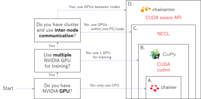
Nowadays it is important for deep learning library to use GPU to enhance its calculation speed, and Chainer provides several levels of GPU support.
The packages which you need to install depends on your PC envitonment, please follow this figure to understand what category you are in.
The chart to specify what you need to install.
Note that the upper category includes the lower dependencies. For example, if you are categorized to B., then you need to install A. chainer and B. Cupy, CUDA, cudnn.
I think most of the users are categorized as A. or B., C. and D. are for only professionals.
A: CPU user
If you don’t have NVIDIA GPU and GPU support is not necessary, you only need to install chainer.
The difference of using GPU (category B., C., D.) is basically only the calculation speed, you can enjoy trying all the functionality of chainer.
※ It is ok to try using chainer with only CPU. But when you want to seriously run deep learning code with big data (such as images etc), you might feel it runs too slow with only CPU.
Install chainer
pip install chainer
Just one line, that’s all :).
Update chainer
Chainer development is very active and its version update is released very often (see Release Cycle for details).
To check the current version: you can type following in command line,
If you have NVIDIA GPU, you can get benefit for calculation enhancement by installing cupy, which is like GPU version of numpy. GPU is good at parallel computing, and once you setup CUDA, cudnn, and cupy it may sometimes more than 10 times faster than using only CPU, depending on the task (for example, CNN used in image processing can get this benefit a lot!).
Before installing cupy, you need to install/setup CUDA and cudnn library.
CUDA® is a parallel computing platform and programming model invented by NVIDIA. It enables dramatic increases in computing performance by harnessing the power of the graphics processing unit (GPU).
Please follow official download page to get CUDA library and install it.
Install cudnn
The NVIDIA CUDA® Deep Neural Network library (cuDNN) is a GPU-accelerated library of primitives for deep neural networks.
Even without cudnn, and only with CUDA, chainer can use GPU calculation. However if you install cudnn, its calculation is more highly optimized. Especially, GPU memory usage reduces dramatically and thus I recommend to install cudnn as well.
Please go to cudnn download page to get cudnn library and install. You might need to register membership to download cudnn library.
Install cupy
pip install cupy
Basically that’s all. See install cupy for details.
When you install CuPy without CUDA, and after that you want to use CUDA, please reinstall CuPy. You need to reinstall CuPy when you want to upgrade CUDA.
Reinstall chainer, cupy
When you reinstall the package, it is better to specify explicitly not to use cached file.
To use this module, you need to install NCCL library.
※ If you are not going to train the model with multiple GPUs, you can skip installing NCCL Even you have multiple GPUs. For example, you can run training process for “model A” with gpu 0, and another training process for “model B” with GPU 1 at the same time without NCCL setup.
Install NCCL
NCCL (pronounced “Nickel”) is a stand-alone library of standard collective communication routines, such as all-gather, reduce, broadcast, etc., that have been optimized to achieve high bandwidth over PCIe.
TL;DR; I recommend to install “anaconda” instead of using “official python package”.
If you just want to proceed environment setup, jump to “Environment setup for each OS”. At first, I will explain little bit about the background knowledge of python & anaconda.
Python version
Python version 2 and 3 are distributed, current latest version is python 2.7 and python 3.6.
Several years ago, it is said that “some library is still not compatible with python 3.x, and thus python 2.x is recommended”. However, now most of the popular library works well with python 3.x.
Here, I recommend to install python 3.x as a default environment, and switch to python 2.7 if necessary using conda‘s virtual environment functionality.
Problems for python development setup
When you use pure system python, you will face following problems. These problems can be solved with anaconda!
Version control: Change python version depending on the project. – Depending on the library you may need to change python2/python3 environment. – When you want to run other person’s code, sometimes it is written in python2 and sometimes in python3. → conda create command to create another environment with specific python version.
Development environment management: – You might want to use developed branch/specific version of library only for specific project. You need to prepare multiple development environment to control python library version. → conda create command to create another environment.
pip install fails with some library for compilation depends on OS: – Especially this happens for Windows users. Some library is only distributed for Linux user and compilation fails when installing with pip command. → Try ‘conda install library-name' to install library.
python 2.x is pre-installed to system on Linux/Mac – How to use python 3.x without conflicting with system python 2.x. → Use pyenv to avoid conflict with system python.
Anaconda is one of the python distribution package, which includes popular libraries from default (numpy, scipy, pandas, ipython, jupyter, scikit-learn etc…).
There is also miniconda, which includes minimum package.
Python version: Both python 2.x and python 3.x version are distributed.
OS support: Linux, Max, Windows version are available, supports both 32 bit & 64 bit.
When you install anaconda package, you can use conda .
Package management: conda is package management tool, which can be considered as an alternative for pip.
It supports over 400 packages
pip tries to compile the package in client environment, and the compile sometimes fails depending on your environment (OS, library etc).
conda provides pre-compiled package, and it reduces install failure case.
It does not interfere with pip command, you can still use pip if the package is not included in conda.
Version control: conda supports python version control, as an alternative for pyenv
For example, you can create python 2.7 virtual environment named ‘py27’ by
conda create -n py27 python=2.7
To enter this virtual environment,
source activate py27
Virtual environment management: as an altenative for virtualenv/venv
Environment setup for each OS
Windows
Python is not pre-installed on windows, you can just install anaconda.
Setup
1. Install anaconda
You can download installer from official anaconda download site. Follow instruction of exe installer, it also manages to add system PATH environment for the convenience.
I recommend to install latest version (anaconda 4.4.0, python 3.6 at the time of writing 2917/6/28), you may create another python version (e.g. python 2.7) virtual environment easily after the installation.
2. Check installation (you may skip this)
Launch command line (Press Windows key, type ‘cmd’ and enter).
Python is pre-installed on system, and it is usually python 2.7. You need to configure to use installed anaconda.
However, if you only install anaconda, it also installs curl, sqlite, openssl and override additional commands, which might cause conflict with existing environment.
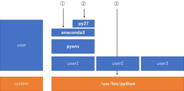
Recommended way is to install anacondaon top of pyenv.
python environment architecture. After the environment setup, user1 can use anaconda3 (python 3) or virtual env py27 (python 2.7), which is independent from pre-installed system python (/usr/bin/python).
See this figure, assuming you are user1.
As default, you can use anaconda3 which is python 3.x.
If you create virtual env (ex, ‘py27’), you can use python 2.7 as well.
It is user-dependent configuration, and does not affect to other user. If other user (user2, user3) did not setup, they will use system python.
This configuration has another advantage that your configuration does not affect to other user, it is good for construct work environment in shared server.
First line clones the package 2nd – 4th line will add necessary environment setup command to .bashrc Last line will initialize system with modified .bashrc
2. Install anaconda: you can install either python 3.x package or python 2.x package.
I think it is ok to install python 3.x version as a default, and you don’t need to install both because python version 2/3 can be switched with conda.
# Check latest version, anaconda3-4.2.0 (anaconda2-4.2.0 for python 2.7)
$ pyenv install -l | grep ana

# Install anaconda, and configure to set anaconda as default python
$ pyenv install anaconda3-4.2.0
$ pyenv rehash
$ pyenv global anaconda3-4.2.0

# set PATH to avoid `activate` command conflict between pyenv and anaconda (use anaconda's activate)
$ echo 'export PATH="$PYENV_ROOT/versions/anaconda3-4.2.0/bin/:$PATH"' >> ~/.bashrc
$ source ~/.bashrc

# update conda itself
$ conda update conda
[Note] If you prefer, you may install miniconda instead of anaconda with the similar procedure.
If python and pip uses anaconda’s command under user’s directory, installation is ok. If it looks system python (python 2.7), installation is not successful.
Mac
I don’t have Mac, sorry. But the basic procedure is same with Linux except that pyenv installation is via homebrew.
conda basic usage
virtual environment
Create virtual env
conda create -n <environment-name> python=<version> <install libraries with space separated>
# Enter virtual env
# `activate py27` for Windows
source activate py27

# Exit virtual env
# `deactivate` for windows
source deactivate
Delete virtual env
conda remove -n py27 --all
package management
Install/uninstall package
# install
conda install numpy scipy  # specify multiple libraries, like pip
conda install numpy=1.10.4 # specify version
conda install -n py2 numpy scipy # -n option to specify virtual env

conda update numpy # update

pip install numpy  # pip can be used as well. Use it when the library is not in conda
source activate py2;pip install numpy # Install library in virtual env, install it after `activate`

# uninstall
conda uninstall -n py2 numpy
Check package
# Show current installed package list
conda list

# -n option to specify virtual env
conda list -n py27

# Export list and use it in another environment
# However, package installed with `pip` cannot be exported.
# use `pip freeze` to output the list of package installed with pip.
conda list --export > env.txt
conda create -n py27_copy --file env.txt
Search package in anaconda cloud
Even the package is not distributed by official anaconda, other third-party may be uploaded to anaconda cloud (anaconda.org).
It is useful to check the package is distributed under anaconda cloud, and install it.
To search,
anaconda search -t conda <package-name-to-search>
And once found, to install third party library,
conda install -c <USER> <PACKAGE>
here <USER> means third party’s name, and <PACKAGE> means the package name to install.
Below example shows how to install rdkit package, which is not distributed under anaconda but by rdkit.
I used the same seed (=13) to extract the train and test data used in the training phase.
Load trained model
# Load trained model
model = MyMLP(args.unit) # type: MyMLP
if args.gpu >= 0:
chainer.cuda.get_device(args.gpu).use() # Make a specified GPU current
model.to_gpu() # Copy the model to the GPU
xp = np if args.gpu < 0 else cuda.cupy
serializers.load_npz(args.modelpath, model)
The procedure to load the trained model is
Instantiate the model (which is a subclass of Chain: here, it is MyMLP)
Send the parameters to GPU if necessary.
Load the trained parameters using serializers.load_npz function.
Predict with minibatch
Prepare minibatch from dataset with concat_examples
We need to feed minibatch instead of dataset itself into the model. The minibatch was constructed by the Iterator in training phase. In predict phase, it might be too much to prepare Iterator, then how to construct minibatch?
There is a convenient function, concat_examples, to prepare minibatch from dataset. It works as written in this figure.
concat_examples converts dataset list into minibatch for each feature (here, x and y) which can be input into neural network.
Usually when we access dataset by slice indexing, for example dataset[i:j], it returns a list where data is sequential. concat_examples separates each element of data and concatenates it to generate minibatch.
You can use as follows,
from chainer.dataset import concat_examples
x, t = concat_examples(test[i:i + batchsize])
y = model.predict(x)
...
Predict phase has some difference compared to training phase,
Function behavior – Expected behavior of some functions are different between training phase and validation/predict phase. For example, F.dropout is expected to drop out some unit in the training phase while it is better to not to drop out in validation/predict phase.These kinds of function behavior is handled by chainer.config.train configuration.
Back propagation is not necessary When back propagation is enabled, the model need to construct computational graph which requires additional memory. However back propagation is not necessary in validation/predict phase and we can omit constructing computational graph to reduce memory usage.
This can be controlled by chainer.config.enable_backprop, and chainer.no_backprop_mode() function can be used for convenient method.
By considering above, we can write predict code in the MyMLP model as,
class MyMLP(chainer.Chain):
...
def predict(self, *args):
with chainer.using_config('train', False):
with chainer.no_backprop_mode():
return self.forward(*args)
Finally, predict code can be written as follows,
# Predict
x_list = []
y_list = []
t_list = []
for i in range(0, len(test), batchsize):
x, t = concat_examples(test[i:i + batchsize])
y = model.predict(x)
y_list.append(y.data)
x_list.append(x)
t_list.append(t)
x_test = np.concatenate(x_list)[:, 0]
y_test = np.concatenate(y_list)[:, 0]
t_test = np.concatenate(t_list)[:, 0]
print('x', x_test)
print('y', y_test)
print('t', t_test)
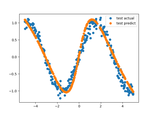
Plot the result
This is a regression task, so let’s see the difference between actual point and model’s predicted point.
Move predict function into model class: if you want to simplify main predict code in predict_custom_dataset1.py, you may move predict for loop into model side.
def predict2(self, *args, batchsize=32):
data = args[0]
x_list = []
y_list = []
t_list = []
for i in range(0, len(data), batchsize):
x, t = concat_examples(data[i:i + batchsize])
y = self.predict(x)
y_list.append(y.data)
x_list.append(x)
t_list.append(t)
x_array = np.concatenate(x_list)[:, 0]
y_array = np.concatenate(y_list)[:, 0]
t_array = np.concatenate(t_list)[:, 0]
return x_array, y_array, t_array
then, we can write main predict code very simply,
"""Inference/predict code for MNIST
model must be trained before inference, train_mnist_4_trainer.py must be executed beforehand.
"""
from __future__ import print_function
import argparse
import time
import numpy as np
import six
import matplotlib.pyplot as plt
import chainer
import chainer.functions as F
import chainer.links as L
from chainer import Chain, Variable, optimizers, serializers
from chainer import datasets, training, cuda, computational_graph
from chainer.dataset import concat_examples
from my_mlp import MyMLP
from my_dataset import MyDataset
def main():
parser = argparse.ArgumentParser(description='Chainer example: MNIST')
parser.add_argument('--modelpath', '-m', default='result/mymlp.model',
help='Model path to be loaded')
parser.add_argument('--gpu', '-g', type=int, default=-1,
help='GPU ID (negative value indicates CPU)')
parser.add_argument('--unit', '-u', type=int, default=50,
help='Number of units')
parser.add_argument('--batchsize', '-b', type=int, default=10,
help='Number of images in each mini-batch')
args = parser.parse_args()
batchsize = args.batchsize
    # Load the custom dataset
    dataset = MyDataset('data/my_data.csv')
    train_ratio = 0.7
    train_size = int(len(dataset) * train_ratio)
    train, test = chainer.datasets.split_dataset_random(dataset, train_size, seed=13)
    # Load trained model
    model = MyMLP(args.unit)  # type: MyMLP
    if args.gpu >= 0:
        chainer.cuda.get_device(args.gpu).use()  # Make a specified GPU current
        model.to_gpu()  # Copy the model to the GPU
    xp = np if args.gpu < 0 else cuda.cupy

    serializers.load_npz(args.modelpath, model)
# Predict
x_test, y_test, t_test = model.predict2(test)
print('x', x_test)
print('y', y_test)
print('t', t_test)
plt.figure()
plt.plot(x_test, t_test, 'o', label='test actual')
plt.plot(x_test, y_test, 'o', label='test predict')
plt.legend()
plt.savefig('predict2.png')
if __name__ == '__main__':
main()
We often use mean squared error as loss function, namely,
$$ L = \frac{1}{D}\sum_i^D (t_i – y_i)^2 $$
where \(i\) denotes i-th data, \(D\) is number of data, and \(y_i\) is model’s output from input \(x_i \).
The implementation for MLP can be written as my_mlp.py,
class MyMLP(chainer.Chain):

    def __init__(self, n_units):
        super(MyMLP, self).__init__()
        with self.init_scope():
            # the size of the inputs to each layer will be inferred
            self.l1 = L.Linear(n_units)  # n_in -> n_units
            self.l2 = L.Linear(n_units)  # n_units -> n_units
            self.l3 = L.Linear(n_units)  # n_units -> n_units
            self.l4 = L.Linear(1)    # n_units -> n_out

    def __call__(self, *args):
        # Calculate loss
        h = self.forward(*args)
        t = args[1]
        self.loss = F.mean_squared_error(h, t)
        reporter.report({'loss': self.loss}, self)
        return self.loss

    def forward(self, *args):
        # Common code for both loss (__call__) and predict
        x = args[0]
        h = F.sigmoid(self.l1(x))
        h = F.sigmoid(self.l2(h))
        h = F.sigmoid(self.l3(h))
        h = self.l4(h)
        return h
In this case, MyMLP model will calculate y (target to predict) in forward computation, and loss is calculated at __call__function of the model.
Data separation for validation/test
When you are downloading publicly available machine learning dataset, it is often separated as training data and test data (and sometimes validation data) from the beginning.
However, our custom dataset is not separated yet. We can split the existing dataset easily with chainer’s function, which includes following function
These are useful to separate training data and test data, example usage is as following,
    # Load the dataset and separate to train data and test data
    dataset = MyDataset('data/my_data.csv')
    train_ratio = 0.7
    train_size = int(len(dataset) * train_ratio)
    train, test = chainer.datasets.split_dataset_random(dataset, train_size, seed=13)
Here, we load our data as dataset (which is subclass of DatasetMixin), and split this dataset into train and test using chainer.datasets.split_dataset_random function. I split train data 70% : test data 30%, randomly in above code.
We can also specify seed argument to fix the random permutation order, which is useful for reproducing experiment or predicting code with same train/test dataset.
from __future__ import print_function
import argparse

import chainer
import chainer.functions as F
import chainer.links as L
from chainer import training
from chainer.training import extensions
from chainer import serializers

from my_mlp import MyMLP
from my_dataset import MyDataset


def main():
    parser = argparse.ArgumentParser(description='Train custom dataset')
    parser.add_argument('--batchsize', '-b', type=int, default=10,
                        help='Number of images in each mini-batch')
    parser.add_argument('--epoch', '-e', type=int, default=20,
                        help='Number of sweeps over the dataset to train')
    parser.add_argument('--gpu', '-g', type=int, default=-1,
                        help='GPU ID (negative value indicates CPU)')
    parser.add_argument('--out', '-o', default='result',
                        help='Directory to output the result')
    parser.add_argument('--resume', '-r', default='',
                        help='Resume the training from snapshot')
    parser.add_argument('--unit', '-u', type=int, default=50,
                        help='Number of units')
    args = parser.parse_args()

    print('GPU: {}'.format(args.gpu))
    print('# unit: {}'.format(args.unit))
    print('# Minibatch-size: {}'.format(args.batchsize))
    print('# epoch: {}'.format(args.epoch))
    print('')

    # Set up a neural network to train
    # Classifier reports softmax cross entropy loss and accuracy at every
    # iteration, which will be used by the PrintReport extension below.
    model = MyMLP(args.unit)

    if args.gpu >= 0:
        chainer.cuda.get_device(args.gpu).use()  # Make a specified GPU current
        model.to_gpu()  # Copy the model to the GPU

    # Setup an optimizer
    optimizer = chainer.optimizers.MomentumSGD()
    optimizer.setup(model)

    # Load the dataset and separate to train data and test data
    dataset = MyDataset('data/my_data.csv')
    train_ratio = 0.7
    train_size = int(len(dataset) * train_ratio)
    train, test = chainer.datasets.split_dataset_random(dataset, train_size, seed=13)

    train_iter = chainer.iterators.SerialIterator(train, args.batchsize)
    test_iter = chainer.iterators.SerialIterator(test, args.batchsize, repeat=False, shuffle=False)

    # Set up a trainer
    updater = training.StandardUpdater(train_iter, optimizer, device=args.gpu)
    trainer = training.Trainer(updater, (args.epoch, 'epoch'), out=args.out)

    # Evaluate the model with the test dataset for each epoch
    trainer.extend(extensions.Evaluator(test_iter, model, device=args.gpu))

    # Dump a computational graph from 'loss' variable at the first iteration
    # The "main" refers to the target link of the "main" optimizer.
    trainer.extend(extensions.dump_graph('main/loss'))

    # Take a snapshot at each epoch
    #trainer.extend(extensions.snapshot(), trigger=(args.epoch, 'epoch'))
    trainer.extend(extensions.snapshot(), trigger=(1, 'epoch'))

    # Write a log of evaluation statistics for each epoch
    trainer.extend(extensions.LogReport())

    # Print selected entries of the log to stdout
    # Here "main" refers to the target link of the "main" optimizer again, and
    # "validation" refers to the default name of the Evaluator extension.
    # Entries other than 'epoch' are reported by the Classifier link, called by
    # either the updater or the evaluator.
    trainer.extend(extensions.PrintReport(
        ['epoch', 'main/loss', 'validation/main/loss', 'elapsed_time']))

    # Plot graph for loss for each epoch
    if extensions.PlotReport.available():
        trainer.extend(extensions.PlotReport(
            ['main/loss', 'validation/main/loss'],
            x_key='epoch', file_name='loss.png'))
    else:
        print('Warning: PlotReport is not available in your environment')
    # Print a progress bar to stdout
    trainer.extend(extensions.ProgressBar())

    if args.resume:
        # Resume from a snapshot
        serializers.load_npz(args.resume, trainer)

    # Run the training
    trainer.run()
    serializers.save_npz('{}/mymlp.model'.format(args.out), model)

if __name__ == '__main__':
    main()
[hands on]
Execute train_custom_dataset.py to train the model. Trained model parameter will be saved to result/mymlp.model.
In previous chapter we have learned how to train deep neural network using MNIST handwritten digits dataset. However, MNIST dataset has prepared by chainer utility library and you might now wonder how to prepare dataset when you want to use your own data for regression/classification task.
Chainer provides DatasetMixin class to let you define your own dataset class.
Prepare Data
In this task, we will try very simple regression task. Own dataset can be generated by create_my_dataset.py.
import os
import numpy as np
import pandas as pd


DATA_DIR = 'data'


def black_box_fn(x_data):
    return np.sin(x_data) + np.random.normal(0, 0.1, x_data.shape)


if __name__ == '__main__':
    if not os.path.exists(DATA_DIR):
        os.mkdir(DATA_DIR)

    x = np.arange(-5, 5, 0.01)
    t = black_box_fn(x)
    df = pd.DataFrame({'x': x, 't': t}, columns={'x', 't'})
    df.to_csv(os.path.join(DATA_DIR, 'my_data.csv'), index=False)
This script will create very simple csv file named “data/my_data.csv“, with column name “x” and “t”. “x” indicates input value and “t” indicates target value to predict.
I adopted simple sin function with a little bit of Gaussian noise to generate “t” from “x”. (You may try modifying black_box_fn function to change the function to estimate.
Our task is to get a regression model of this black_box_fn.
Define MyDataset as a subclass of DatasetMixin
Now you have your own data, let’s define dataset class by inheriting DatasetMixin class provided by chainer.
Implementation
We usually implement 3 functions, such as
__init__(self, *args) To write initialization code.
__len__(self) Trainer module (Iterator) accesses this property to calculate the training progress in epoch.
import numpy as np
import pandas as pd

import chainer


class MyDataset(chainer.dataset.DatasetMixin):

    def __init__(self, filepath, debug=False):
        self.debug = debug
        # Load the data in initialization
        df = pd.read_csv(filepath)
        self.data = df.values.astype(np.float32)
        if self.debug:
            print('[DEBUG] data: \n{}'.format(self.data))

    def __len__(self):
        """return length of this dataset"""
        return len(self.data)

    def get_example(self, i):
        """Return i-th data"""
        x, t = self.data[i]
        return [x], [t]
Most important part is override function, get_example(self, i) where this function should be implemented to return only i-th data.
※ We don’t need to care about minibatch concatenation, Iterator will handle these stuffs. You only need to prepare a dataset to return i-th data :).
The above code works following,
1. We load prepared data ‘data/my_data.csv‘ (set as filepath) in __init__ function in the initialization code, and set expanded array (strictly, pandas.DataFrame class) into self.data.
2. return i-th data xi and ti as a vector with size 1 in get_example(self, i).
How does it work
The idea is simple. You can instantiate dataset with MyDataset() and then you can access i-th data by dataset[i].
It is also possible to access by slice or one dimensional vector, dataset[i:j] returns [dataset[i], dataset[i+1], …, dataset[j-1]].
if __name__ == '__main__':
    # Test code
    dataset = MyDataset('data/my_data.csv', debug=True)

    print('Access by index dataset[1] = ', dataset[1])
    print('Access by slice dataset[:3] = ', dataset[:3])
    print('Access by list dataset[[3, 5]] = ', dataset[[3, 5]])
    index = np.arange(3)
    print('Access by numpy array dataset[[0, 1, 2]] = ', dataset[index])
    # Randomly take 3 data
    index = np.random.permutation(len(dataset))[:3]
    print('dataset[{}] = {}'.format(index, dataset[index]))
Flexibility of DatasetMixin – dynamic load from stolage, preprocess, data augmentation
(This my be advanced topic for now. You may skip and come back later.)
The nice part of DatasetMixin class is its flexibility. Basically you can implement anything in get_example function, and get_example is called every time when we access the data with data[i].
1. Data augmentation
This means we can write dynamic preprocessing. For example data augmentation is wll known, important Technic to avoid overfitting and get high validation score especially in image processing.
See chainer official imagenet example for the reference.
If you are dealing with very big size data, and all data cannot be expanded in memory at once, the best practice is to load the data each time when necessary (when creating minibatch).
We can achieve this procedure easy with DatasetMixin class. Simply, you can write loading code in get_example function to load i-th data from storage that’s all!
First, construct the model and load the trained model parameters,
    # Model Setup
    model = archs[args.arch](n_vocab=N_VOCABULARY, n_units=args.unit)
    if args.gpu >= 0:
        chainer.cuda.get_device(args.gpu).use()  # Make a specified GPU current
        model.to_gpu()                           # Copy the model to the GPU
    xp = np if args.gpu < 0 else cuda.cupy

    serializers.load_npz(args.modelpath, model)
Then we only specify the first index (corresponds to word id), primeindex, and generate next index. We can generate next index repeatedly based on the generated index.
    # Predict
    predicted_sequence = [prev_index]
    for i in range(args.length):
        prev = chainer.Variable(xp.array([prev_index], dtype=xp.int32))
        current = model(prev)
        current_index = np.argmax(cuda.to_cpu(current.data))
        predicted_sequence.append(current_index)
        prev_index = current_index

    print('Predicted sequence: ', predicted_sequence)
The result is the following, successfully generate the sequence.
This is a simple example to check if RNN has an ability to remember past sequence, so I didn’t prepare validation data. I just wanted to check if the RNN model can “memorize” the training data sequence or not.
Note that the situation is little bit different during training phase and inference/predict phase. In training phase, the model is trained to generate \(xt\) based on the correct sequence \([x_0, x_1, \dots, x_{t-1}]\).
However in predict phase, we only specify the first index \(x_0\), and the model will generate \(x’_1\) (here ‘ indicates output from the model). After that, the model need to generate \(x’_2\) based on \(x’_1\). Therefore, the model will generate \(x’_t\) based on the predicted sequence \([x_0, x’_1 \dots, x’_{t-1}]\).
CuPy module becomes independent. Reason is that CuPy is GPU version of numpy, it can be used for many types of linear calculation, not specific for chainer.
If you are using only CPU, this is enough as previous
pip install chainer
If you want to get a benefit of GPU, you need to setup CUDA and need to install CuPy separately.
pip install chainer
pip install cupy
[NOTE] Also, is you have multiple GPU, you can install NCCL before install chainer and cupy to use MultiProcessParallelUpdater.
Important to note that NO source code change is necessary for your Chainer development. Chainer will import CuPy only when it is installed in your environment.
Global configuration is introduced
Global config chainer.global_config and thread local config chainer.config is introduced to control the chainer behavior.
Function behavior can be controlled by using chainer.config.train flag instead of writing it in function argument. I will just cite above official doc for the example,
Example
Consider the following model definition and the code to call it in test mode written for Chainer v1.
# Chainer v1
import chainer.functions as F
class MyModel(chainer.Link):
    ...

    def __call__(self, x, train=True):
        return f(F.dropout(x, train=train))
m = MyModel(...)
y = m(x, train=False)
In Chainer v2, it should be updated into the following code:
# Chainer v2
import chainer.functions as F
class MyModel(chainer.Link):
    ...

    def __call__(self, x):
        return f(F.dropout(x))
m = MyModel(...)
with chainer.using_config('train', False):
    y = m(x)
When you define your own Link or Chain class, init_scope() can be used to initialize Parameter or Link,
This writing style is recommended because of IDE (PyCharm etc) can enhance the local variable indexing and show type hinting. But you can still use conventional (chainer v1) initialization as well.
Below is an example of defining Chain class, from official doc,
Example
For example, the following chain initialization code
We have learned in previous post that RNN is expected to have an ability to remember the sequence information. Let’s do a easy experiment to check it before trying actual NLP application.
Simple sequence dataset
I just prepared a simple script to generate simple integer sequence as follows,
import numpy as np

N_VOCABULARY = 10

def get_simple_sequence(n_vocab, repeat=100):
    data = []
    for i in range(repeat):
        for j in range(n_vocab):
            for k in range(j):
                data.append(j)

    return np.asarray(data, dtype=np.int32)

if __name__ == '__main__':
    data = get_simple_sequence(N_VOCABULARY)
    print(data)
So the number i is repeated i times. In order for RNN to generate correct sequence, RNN need to “count” how many times this number already appeared.
For example, to output correct sequence of 9 9 9 … followed by 1, RNN need to count if 9 is already appeared 9 times to output 1.
Training code for RNN
Training procedure of RNN is little bit complicated compared to MLP or CNN, due to the existence of recurrent loop and we need to deal with back propagation with sequential data properly.
To achieve this, we implement custom iterator and updater.
When training RNN, we need to input the data sequentially. Thus we should not take random permutation. We need to be careful when creating the minibatch dataset so that each minibatch should be feed in sequence.
You can implement custom Iterator class to achieve this functionality. The parent class Iterator is implemented as following, Iterator code.
So what we need to implement in Iterator is
__init__(self, ...) : Initialization code.
__next__(self) : This is the core part of iterator. For each iteration, this function is automatically called to get next minibatch.
epoch_detail(self) : This property is used by trainer module to show the progress of training.
serialize(self) : Implement if you want to support resume functionality of trainer.
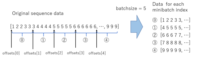
We will implement ParallelSequentialIterator, works following, please also see the figure above.
It will get dataset in the __init__ code, and split the dataset equally with size batch_size.
Every iteration of the training loop, __next__() is called. This iterator will prepare current word (input data) and next word (answer data). The RNN model is trained to predict next word from current word (and its recurrent unit, which encodes the past sequence information).
Additionally, in order for the trainer extensions to work nicely, epoch_detail and serialize are implemented. (These are not mandatory for minimum implementation.)
"""
This code is copied from official chainer examples
 - https://github.com/chainer/chainer/blob/e2fe6f8023e635f8c1fc9c89e85d075ebd50c529/examples/ptb/train_ptb.py
"""
import chainer


# Dataset iterator to create a batch of sequences at different positions.
# This iterator returns a pair of current words and the next words. Each
# example is a part of sequences starting from the different offsets
# equally spaced within the whole sequence.
class ParallelSequentialIterator(chainer.dataset.Iterator):

    def __init__(self, dataset, batch_size, repeat=True):
        self.dataset = dataset
        self.batch_size = batch_size  # batch size
        # Number of completed sweeps over the dataset. In this case, it is
        # incremented if every word is visited at least once after the last
        # increment.
        self.epoch = 0
        # True if the epoch is incremented at the last iteration.
        self.is_new_epoch = False
        self.repeat = repeat
        length = len(dataset)
        # Offsets maintain the position of each sequence in the mini-batch.
        self.offsets = [i * length // batch_size for i in range(batch_size)]
        # NOTE: this is not a count of parameter updates. It is just a count of
        # calls of ``__next__``.
        self.iteration = 0

    def __next__(self):
        # This iterator returns a list representing a mini-batch. Each item
        # indicates a different position in the original sequence. Each item is
        # represented by a pair of two word IDs. The first word is at the
        # "current" position, while the second word at the next position.
        # At each iteration, the iteration count is incremented, which pushes
        # forward the "current" position.
        length = len(self.dataset)
        if not self.repeat and self.iteration * self.batch_size >= length:
            # If not self.repeat, this iterator stops at the end of the first
            # epoch (i.e., when all words are visited once).
            raise StopIteration
        cur_words = self.get_words()
        self.iteration += 1
        next_words = self.get_words()

        epoch = self.iteration * self.batch_size // length
        self.is_new_epoch = self.epoch < epoch
        if self.is_new_epoch:
            self.epoch = epoch

        return list(zip(cur_words, next_words))

    @property
    def epoch_detail(self):
        # Floating point version of epoch.
        return self.iteration * self.batch_size / len(self.dataset)

    def get_words(self):
        # It returns a list of current words.
        return [self.dataset[(offset + self.iteration) % len(self.dataset)]
                for offset in self.offsets]

    def serialize(self, serializer):
        # It is important to serialize the state to be recovered on resume.
        self.iteration = serializer('iteration', self.iteration)
        self.epoch = serializer('epoch', self.epoch)
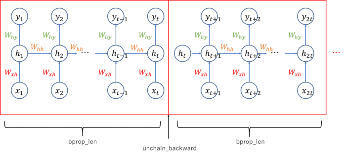
Updater – Truncated back propagation through time (BPTT)
Truncated Backpropagation Through Time. For RNN, each forward computation (arrow from bottom to top) depends on the previous recurrent unit. Thus we need to compute forward computation several times to proceed to backward computation.
Back propagation through time: The training procedure for RNN model is different from MLP or CNN. Because each forward computation of RNN depends on the previous forward computation due to the existence of recurrent unit. Therefore we need to execute forward computation several times before executing backward computation to allow recurrent loop, Whh, to learn the sequential information. We set the value bprop_len (back propagation length) in below Updater implementation. Forward computation is executed this number of times consecutively, followed by one time of back propagation.
Truncate computational graph: Also, as you can see from the above figure, RNN graph will grow every time the forward computation is executed, and computer cannot handle if the graph grows infinitely long. To deal with this issue, we will cut (truncate) the graph after each time of backward computation. It can be achieved by calling unchain_backward function in chainer.
This optimization method can be implemented by creating custom Updater class, BPTTUpdater, as a subclass of StandardUpdater.
It just overrides the function update_core, which is the function to write parameter update (optimize) process.
“”” This code is copied from official chainer examples
https://github.com/chainer/chainer/blob/e2fe6f8023e635f8c1fc9c89e85d075ebd50c529/examples/ptb/train_ptb.py “”” import chainer from chainer import training
Custom updater for truncated BackProp Through Time (BPTT)
class BPTTUpdater(training.StandardUpdater):
def __init__(self, train_iter, optimizer, bprop_len, device):
    super(BPTTUpdater, self).__init__(
        train_iter, optimizer, device=device)
    self.bprop_len = bprop_len

# The core part of the update routine can be customized by overriding.
def update_core(self):
    loss = 0
    # When we pass one iterator and optimizer to StandardUpdater.__init__,
    # they are automatically named 'main'.
    train_iter = self.get_iterator('main')
    optimizer = self.get_optimizer('main')

    # Progress the dataset iterator for bprop_len words at each iteration.
    for i in range(self.bprop_len):
        # Get the next batch (a list of tuples of two word IDs)
        batch = train_iter.__next__()

        # Concatenate the word IDs to matrices and send them to the device
        # self.converter does this job
        # (it is chainer.dataset.concat_examples by default)
        x, t = self.converter(batch, self.device)

        # Compute the loss at this time step and accumulate it
        loss += optimizer.target(chainer.Variable(x), chainer.Variable(t))

    optimizer.target.cleargrads()  # Clear the parameter gradients
    loss.backward()  # Backprop
    loss.unchain_backward()  # Truncate the graph
    optimizer.update()  # Update the parameters
As you can see, forward is executed in the for loop bprop_len times consecutively to accumulate loss, followed by one backward to execute the back propagation of this accumulated loss. After that, the parameter is updated by optimizer using update funciton.
Note that unchain_backward is called every time at the end of the update_core function to truncate/cut the computational graph.
Main training code
Once iterator and the updater are prepared, training code is almost same with previous training for MLP-MNIST task or CNN-CIFAR10/CIFAR100.
"""
RNN Training code with simple sequence dataset
"""
from __future__ import print_function

import os
import sys
import argparse

import matplotlib
matplotlib.use('Agg')
import matplotlib.pyplot as plt

import chainer
import chainer.functions as F
import chainer.links as L
from chainer import training, iterators, serializers, optimizers
from chainer.training import extensions

sys.path.append(os.pardir)
from RNN import RNN
from RNN2 import RNN2
from RNN3 import RNN3
from RNNForLM import RNNForLM
from simple_sequence.simple_sequence_dataset import N_VOCABULARY, get_simple_sequence
from parallel_sequential_iterator import ParallelSequentialIterator
from bptt_updater import BPTTUpdater


def main():
    archs = {
        'rnn': RNN,
        'rnn2': RNN2,
        'rnn3': RNN3,
        'lstm': RNNForLM
    }

    parser = argparse.ArgumentParser(description='RNN example')
    parser.add_argument('--arch', '-a', choices=archs.keys(),
                        default='rnn', help='Net architecture')
    parser.add_argument('--unit', '-u', type=int, default=100,
                        help='Number of RNN units in each layer')
    parser.add_argument('--bproplen', '-l', type=int, default=20,
                        help='Number of words in each mini-batch '
                             '(= length of truncated BPTT)')
    parser.add_argument('--batchsize', '-b', type=int, default=10,
                        help='Number of images in each mini-batch')
    parser.add_argument('--epoch', '-e', type=int, default=10,
                        help='Number of sweeps over the dataset to train')
    parser.add_argument('--gpu', '-g', type=int, default=-1,
                        help='GPU ID (negative value indicates CPU)')
    parser.add_argument('--out', '-o', default='result',
                        help='Directory to output the result')
    parser.add_argument('--resume', '-r', default='',
                        help='Resume the training from snapshot')
    args = parser.parse_args()

    print('GPU: {}'.format(args.gpu))
    print('# Architecture: {}'.format(args.arch))
    print('# Minibatch-size: {}'.format(args.batchsize))
    print('# epoch: {}'.format(args.epoch))
    print('')

    # 1. Setup model
    #model = archs[args.arch](n_vocab=N_VOCABRARY, n_units=args.unit)  # activation=F.leaky_relu
    model = archs[args.arch](n_vocab=N_VOCABULARY,
                             n_units=args.unit)  # , activation=F.tanh
    classifier_model = L.Classifier(model)

    if args.gpu >= 0:
        chainer.cuda.get_device(args.gpu).use()  # Make a specified GPU current
        classifier_model.to_gpu()  # Copy the model to the GPU

    eval_classifier_model = classifier_model.copy()  # Model with shared params and distinct states
    eval_model = classifier_model.predictor

    # 2. Setup an optimizer
    optimizer = optimizers.Adam(alpha=0.0005)
    #optimizer = optimizers.MomentumSGD()
    optimizer.setup(classifier_model)

    # 3. Load dataset
    train = get_simple_sequence(N_VOCABULARY)
    test = get_simple_sequence(N_VOCABULARY)

    # 4. Setup an Iterator
    train_iter = ParallelSequentialIterator(train, args.batchsize)
    test_iter = ParallelSequentialIterator(test, args.batchsize, repeat=False)

    # 5. Setup an Updater
    updater = BPTTUpdater(train_iter, optimizer, args.bproplen, args.gpu)
    # 6. Setup a trainer (and extensions)
    trainer = training.Trainer(updater, (args.epoch, 'epoch'), out=args.out)

    # Evaluate the model with the test dataset for each epoch
    trainer.extend(extensions.Evaluator(test_iter, eval_classifier_model,
                                        device=args.gpu,
                                        # Reset the RNN state at the beginning of each evaluation
                                        eval_hook=lambda _: eval_model.reset_state())
                   )

    trainer.extend(extensions.dump_graph('main/loss'))
    trainer.extend(extensions.snapshot(), trigger=(1, 'epoch'))
    trainer.extend(extensions.LogReport())
    trainer.extend(extensions.PrintReport(
        ['epoch', 'main/loss', 'validation/main/loss',
         'main/accuracy', 'validation/main/accuracy', 'elapsed_time']))
    trainer.extend(extensions.PlotReport(
        ['main/loss', 'validation/main/loss'],
        x_key='epoch', file_name='loss.png'))
    trainer.extend(extensions.PlotReport(
        ['main/accuracy', 'validation/main/accuracy'],
        x_key='epoch',
        file_name='accuracy.png'))

    # trainer.extend(extensions.ProgressBar())

    # Resume from a snapshot
    if args.resume:
        serializers.load_npz(args.resume, trainer)

    # Run the training
    trainer.run()
    serializers.save_npz('{}/{}_simple_sequence.model'
                         .format(args.out, args.arch), model)

if __name__ == '__main__':
    main()
Run the code
You can execute the code like,
python train_simple_sequence.py
You can also train with different model using -a option,
python train_simple_sequence.py -a rnn2
Below is the result in my environment with RNN architecture,
I set the N_VOCABULARY=10 in simple_sequence_dataset.py, and even the simple RNN achieved the accuracy close to 1. It seems this RNN model have an ability to remember past 10 sequence.


