[Update 2017.06.11] Add Chainer v2 code.
This post is just a copy of chainer_module1.ipynb on github, you can execute interactively using jupyter notebook.
Advanced memo is written as “Note”. You can skip reading this for the first time reading.
In this tutorial, basic chainer modules are introduced and explained
- Variable
- Link
- Function
- Chain
For other chainer modules are explained in later tutorial.
Initial setup
Below is typecal import statement of chainer modules.
# Initial setup following http://docs.chainer.org/en/stable/tutorial/basic.html
import numpy as np
import chainer
from chainer import cuda, Function, gradient_check, report, training, utils, Variable
from chainer import datasets, iterators, optimizers, serializers
from chainer import Link, Chain, ChainList
import chainer.functions as F
import chainer.links as L
from chainer.training import extensions
Variable
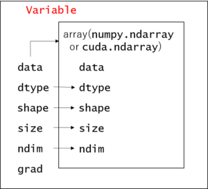
Chainer variable can be created by Variable constructor, which creates chainer.Variable class object.
When I write Variable, it means chainer’s class for Variable. Please do not confuse with the usual noun of “variable”.
Note: the reason why chainer need to use own Variable, Function class for the calculation instead of just using numpy is because back propagation is necessary during deep learning training. Variable holds its “calculation history” information and Function has backward method which is differencial function in order to process back propagation. See below for more details
- Chainer Tutorial Forward/Backward Computation
from chainer import Variable
# creating numpy array
# this is `numpy.ndarray` class
a = np.asarray([1., 2., 3.], dtype=np.float32)

# chainer variable is created from `numpy.ndarray` or `cuda.ndarray` (explained later)
x = Variable(a)

print('a: ', a, ', type: ', type(a))
print('x: ', x, ', type: ', type(x))
a: [ 1. 2. 3.] , type: <class 'numpy.ndarray'>
x: <var@1b45519df60> , type: <class 'chainer.variable.Variable'>
In the above code, numpy data type is explicitly set as dtype=np.float32. If we don’t set data type, np.float64 may be used as default type in 64-bit environment. However such a precision is usually “too much” and not necessary in machine learning. It is better to use lower precision for computational speed & memory usage.
attribute
Chainer Variable has following attributes
- data
- dtype
- shape
- ndim
- size
- grad
They are very similar to numpy.ndarray. You can access following attributes.
# These attributes return the same

print('attributes', 'numpy.ndarray a', 'chcainer.Variable x')
print('dtype', a.dtype, x.dtype)
print('shape', a.shape, x.shape)
print('ndim', a.ndim, x.ndim)
print('size', a.size, x.size)
attributes numpy.ndarray a chcainer.Variable x
dtype float32 float32
shape (3,) (3,)
ndim 1 1
size 3 3
# Variable class has debug_print function, to show this Variable's properties.
x.debug_print()
"<variable at 0x1b45519df60>\n- device: CPU\n- volatile: OFF\n- backend: <class 'numpy.ndarray'>\n- shape: (3,)\n- dtype: float32\n- statistics: mean=2.00000000, std=0.81649661\n- grad: None"
One exception is data attribute, chainer Variable‘s data refers numpy.ndarray
# x = Variable(a)

# `a` can be accessed via `data` attribute from chainer `Variable`
print('x.data is a : ', x.data is a)  # True -> means the reference of x.data and a are same.
print('x.data: ', x.data)
x.data is a :  True
x.data:  [ 1.  2.  3.]
Function
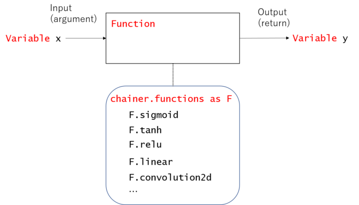
We want to process some calculation to Variable. Variable can be calculated using
- arithmetric operation (Ex.
+,-,*,/) - method which is subclass of
chainer.Function(Ex.F.sigmoid,F.relu)
# Arithmetric operation example
x = Variable(np.array([1, 2, 3], dtype=np.float32))
y = Variable(np.array([5, 6, 7], dtype=np.float32))

# usual arithmetric operator (this case `*`) can be used for calculation of `Variable`
z = x * y
print('z: ', z.data, ', type: ', type(z))
z: [ 5. 12. 21.] , type: <class 'chainer.variable.Variable'>
Only basic calculation can be done with arithmetric operations.
Chainer provides a set of widely used functions via chainer.functions, for example sigmoid function or ReLU (Rectified Linear Unit) function which is popularly used as activation function in deep learning.
# Functoin operation example
import chainer.functions as F

x = Variable(np.array([-1.5, -0.5, 0, 1, 2], dtype=np.float32))
sigmoid_x = F.sigmoid(x)  # sigmoid function. F.sigmoid is subclass of `Function`
relu_x = F.relu(x)        # ReLU function. F.relu is subclass of `Function`

print('x: ', x.data, ', type: ', type(x))
print('sigmoid_x: ', sigmoid_x.data, ', type: ', type(sigmoid_x))
print('relu_x: ', relu_x.data, ', type: ', type(relu_x))
x:  [-1.5 -0.5  0.   1.   2. ] , type:  <class 'chainer.variable.Variable'>
sigmoid_x:  [ 0.18242553  0.37754068  0.5         0.7310586   0.88079709] , type:  <class 'chainer.variable.Variable'>
relu_x:  [ 0.  0.  0.  1.  2.] , type:  <class 'chainer.variable.Variable'>
Note: You can find capital letter of Function like F.Sigmoid or F.ReLU. Basically, these capital letter is actual class implmentation of Function while small letter method is getter method of these capital lettered instance.
It is recommended to use small letter method when you use F.xxx.
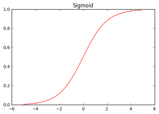
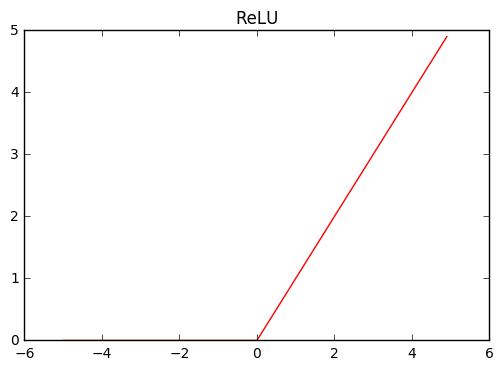
Just a side note, sigmoid and ReLU function are non-linear function whose form is like this.
%matplotlib inline
import matplotlib.pyplot as plt


def plot_chainer_function(f, xmin=-5, xmax=5, title=None):
    """draw graph of chainer `Function` `f`

    :param f: function to be plotted
    :type f: chainer.Function
    :param xmin: int or float, minimum value of x axis
    :param xmax: int or float, maximum value of x axis
    :return:
    """
    a = np.arange(xmin, xmax, step=0.1)
    x = Variable(a)
    y = f(x)
    plt.clf()
    plt.figure()
    # x and y are `Variable`, their value can be accessed via `data` attribute
    plt.plot(x.data, y.data, 'r')
    if title is not None:
        plt.title(title)
    plt.show()

plot_chainer_function(F.sigmoid, title='Sigmoid')
plot_chainer_function(F.relu, title='ReLU')
Link
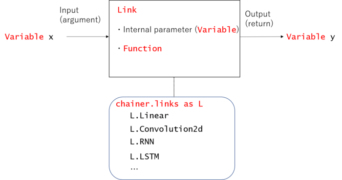
Link is similar to Function, but it owns internal parameter. This internal parameter is tuned during training of machine learning.
Link is similar notion of Layer in caffe. Chainer provides layers which is introduced in popular papers via chainer.links. For example, Linear layer, Convolutional layer.
Let’s see the example, (below explanation is almost same with official tutorial)

import chainer.links as L

in_size = 3  # input vector's dimension
out_size = 2  # output vector's dimension

linear_layer = L.Linear(in_size, out_size)  # L.linear is subclass of `Link`

"""linear_layer has 2 internal parameters `W` and `b`, which are `Variable`"""
print('W: ', linear_layer.W.data, ', shape: ', linear_layer.W.shape)
print('b: ', linear_layer.b.data, ', shape: ', linear_layer.b.shape)
W:  [[-0.11581965  0.44105673 -0.15657252]
 [-0.16952933 -0.57037091 -0.57939512]] , shape:  (2, 3)
b:  [ 0.  0.] , shape:  (2,)
Note that internal parameter W is initialized with a random value. So every time you execute above code, the result will be different (try and check it!).
This Linear layer will take 3-dimensional vectors [x0, x1, x2…] (Variable class) as input and outputs 2-dimensional vectors [y0, y1, y2…] (Variable class).
In equation form, where
where i = 0, 1, 2... denotes each “minibatch” of input/output.
[Note] See source code of Linear class, you can easily understand it is just calling F.linear by
return linear.linear(x, self.W, self.b)
x0 = np.array([1, 0, 0], dtype=np.float32)
x1 = np.array([1, 1, 1], dtype=np.float32)

x = Variable(np.array([x0, x1], dtype=np.float32))
y = linear_layer(x)
print('W: ', linear_layer.W.data)
print('b: ', linear_layer.b.data)
print('x: ', x.data)  # input is x0 & x1
print('y: ', y.data)  # output is y0 & y1
W:  [[-0.11581965  0.44105673 -0.15657252]
 [-0.16952933 -0.57037091 -0.57939512]]
b:  [ 0.  0.]
x:  [[ 1.  0.  0.]
 [ 1.  1.  1.]]
y:  [[-0.11581965 -0.16952933]
 [ 0.16866457 -1.31929541]]
Let me emphasize the difference between Link and Function. Functions input-output relationship is fixed. On the other hand,Link` module has internal parameter and the function behavior can be changed by modifying (tuning) this internal parameter.
# Force update (set) internal parameters
linear_layer.W.data = np.array([[1, 2, 3], [0, 0, 0]], dtype=np.float32)
linear_layer.b.data = np.array([3, 5], dtype=np.float32)

# below is same code with above cell, but output data y will be different
x0 = np.array([1, 0, 0], dtype=np.float32)
x1 = np.array([1, 1, 1], dtype=np.float32)

x = Variable(np.array([x0, x1], dtype=np.float32))
y = linear_layer(x)
print('W: ', linear_layer.W.data)
print('b: ', linear_layer.b.data)
print('x: ', x.data)  # input is x0 & x1
print('y: ', y.data)  # output is y0 & y1
W:  [[ 1.  2.  3.]
 [ 0.  0.  0.]]
b:  [ 3.  5.]
x:  [[ 1.  0.  0.]
 [ 1.  1.  1.]]
y:  [[ 4.  5.]
 [ 9.  5.]]
| 1234567 | W: [[ 1. 2. 3.] [ 0. 0. 0.]]b: [ 3. 5.]x: [[ 1. 0. 0.] [ 1. 1. 1.]]y: [[ 4. 5.] [ 9. 5.]] |
The value of output y is different compared to above code, even though we input same value of x.
These internal parameters are “tuned” during training in machine learning. Usually, we do not need to set these internal parameter W or b manually, chainer will automatically update these internal parameters during training through back propagation.
Chain
Chain is to construct neural networks. It usually consists of several combination of Link and Function modules.
Let’s see example,
from chainer import Chain, Variable


# Defining your own neural networks using `Chain` class
class MyChain(Chain):
    def __init__(self):
        super(MyChain, self).__init__()
        with self.init_scope():
            self.l1 = L.Linear(2, 2)
            self.l2 = L.Linear(2, 1)

    def __call__(self, x):
        h = self.l1(x)
        return self.l2(h)


x = Variable(np.array([[1, 2], [3, 4]], dtype=np.float32))

model = MyChain()
y = model(x)

print('x: ', x.data)  # input is x0 & x1
print('y: ', y.data)  # output is y0 & y1
x:  [[ 1.  2.]
 [ 3.  4.]]
y:  [[-0.54882193]
 [-1.15839911]]
Memo:
Above init_scope() method is introduced in chainer v2,
and Link class instances are initialized inside this scope.
In chainer v1, Chain was initialized as follows.
Concretely, Link class instances are initialized in the argument of super method.
For backward compatibility, you may use this type of initialization in chainer v2 as well.
from chainer import Chain, Variable


# Defining your own neural networks using `Chain` class
class MyChain(Chain):
    def __init__(self):
        super(MyChain, self).__init__(
            l1=L.Linear(2, 2),
            l2=L.Linear(2, 1)
        )

    def __call__(self, x):
        h = self.l1(x)
        return self.l2(h)


x = Variable(np.array([[1, 2], [3, 4]], dtype=np.float32))

model = MyChain()
y = model(x)

print('x: ', x.data)  # input is x0 & x1
print('y: ', y.data)  # output is y0 & y1
x:  [[ 1.  2.]
 [ 3.  4.]]
y:  [[-0.54882193]
 [-1.15839911]]
Based on the official doc, Chain class provides following functionality
- parameter management
- CPU/GPU migration support
- save/load features
to provide convinient reusability of your neural network code.
I will use the word “model” to denote this neural network, implemented as Chain class in Chainer.
Proceed to Chainer basic module introduction 2 to learn how to write “training” code of model, using Optimizer and Serializer.