[Update 2017.06.11] Add chainer v2 code
How can we deal with the sequential data in deep neural network?
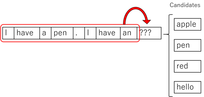
This formulation is especially important in natural language processing (NLP) field. For example, text is made of sequence of word. If we want to predict the next word from given sentence, the probability of the next word depends on whole past sequence of word.
So, the neural network need an ability to “remember” the past sentence to predict next word.
In this chapter, Recurrent Neural Network (RNN) and Long Short Term Memory (LSTM) are introduced to deal with sequential data.
Recurrent Neural Network (RNN)
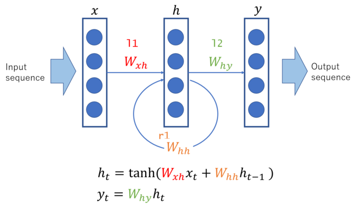
Recurrent Neural Network is similar to Multi Layer Perceptron introduced before, but a loop is added in its hidden layer (Shown in above figure with \( W_{hh} \)).
Here the subscript \(t\) represents the time step (sequence index). Due to this loop hidden layer unit \(h_{t-1}\) is fed again to construct hidden unit \(h_{t}\) of next sequence. Therefore, information of past sequence can be “stored” (memorized) in hidden layer and passed to next sequence.
You might wonder how the loop works in neural network in the above figure, below figure is the expanded version which explicitly explain how the loop works.
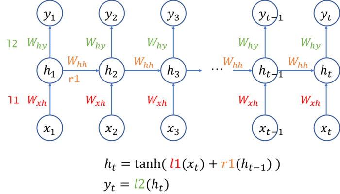
In this figure, data flow is from bottom (\(x\)) to top (\(y\)) and horizontal axis represents time step from left (time step=1) to right (time step=\(t\)).
Every time of the forward computation, it depends on the previous hidden unit \(h_{t-1} \). So the RNN need to keep this hidden unit as a state, see implementation below.
Also, we need to be careful when executing back propagation, because it depends on the history of consecutive forward computation. The detail will be explained in later.
RNN implementation in Chainer
Below code shows implementation of the most simple RNN implementation with one hidden (recurrent) layer, drawn in above figure.
- Source code: RNN.py
import chainer
import chainer.functions as F
import chainer.links as L


class RNN(chainer.Chain):
    """Simple Recurrent Neural Network implementation"""
    def __init__(self, n_vocab, n_units):
        super(RNN, self).__init__()
        with self.init_scope():
            self.embed = L.EmbedID(n_vocab, n_units)
            self.l1 = L.Linear(n_units, n_units)
            self.r1 = L.Linear(n_units, n_units)
            self.l2 = L.Linear(n_units, n_vocab)
        self.recurrent_h = None

    def reset_state(self):
        self.recurrent_h = None

    def __call__(self, x):
        h = self.embed(x)
        if self.recurrent_h is None:
            self.recurrent_h = F.tanh(self.l1(h))
        else:
            self.recurrent_h = F.tanh(self.l1(h) + self.r1(self.recurrent_h))
        y = self.l2(self.recurrent_h)
        return y
EmbedID link
L.EmbedID is used in the above RNN implementation. This is convenient method if you want to input data which can be represented as ID.
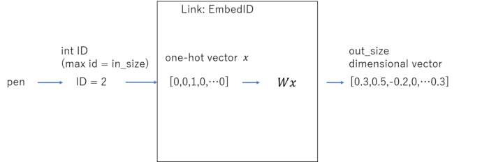
In NLP with text processing, each word is represented as ID in integer. EmbedID layer convert this id into vector which can be considered as vector representation of the word.
More precisely, EmbedID layer works as combination of 2 operations:
- Convert integer ID into
in_sizedimensional one-hot vector. - Apply
Linearlayer (with bias \(b = 0\)) to this one-hot vector to outputout_sizeunits.
See official document for details,
Creating RecurrentBlock as sub-module
If you want to create more deep RNN, you can make recurrent block as a sub module layer like below.
- Source code: RNN2.py
import chainer
import chainer.functions as F
import chainer.links as L


class RecurrentBlock(chainer.Chain):
    """Subblock for RNN"""
    def __init__(self, n_in, n_out, activation=F.tanh):
        super(RecurrentBlock, self).__init__()
        with self.init_scope():
            self.l = L.Linear(n_in, n_out)
            self.r = L.Linear(n_in, n_out)
        self.rh = None
        self.activation = activation

    def reset_state(self):
        self.rh = None

    def __call__(self, h):
        if self.rh is None:
            self.rh = self.activation(self.l(h))
        else:
            self.rh = self.activation(self.l(h) + self.r(self.rh))
        return self.rh


class RNN2(chainer.Chain):
    """RNN implementation using RecurrentBlock"""
    def __init__(self, n_vocab, n_units, activation=F.tanh):
        super(RNN2, self).__init__()
        with self.init_scope():
            self.embed = L.EmbedID(n_vocab, n_units)
            self.r1 = RecurrentBlock(n_units, n_units, activation=activation)
            self.r2 = RecurrentBlock(n_units, n_units, activation=activation)
            self.r3 = RecurrentBlock(n_units, n_units, activation=activation)
            #self.r4 = RecurrentBlock(n_units, n_units, activation=activation)
            self.l5 = L.Linear(n_units, n_vocab)


    def reset_state(self):
        self.r1.reset_state()
        self.r2.reset_state()
        self.r3.reset_state()
        #self.r4.reset_state()

    def __call__(self, x):
        h = self.embed(x)
        h = self.r1(h)
        h = self.r2(h)
        h = self.r3(h)
        #h = self.r4(h)
        y = self.l5(h)
        return y